axis([xmin xmax ymin ymax])axis([xmin xmax ymin ymax zmin zmax])axis autoaxis(axis)v = axis;axis ijaxis xyaxis squareaxis equalaxis offaxis on[s1,s2,s3] = axis('state')
axis provides an easy way to manipulate the most important properties of axes.
axis([xmin xmax ymin ymax]) sets the scaling for the x- and y-axes on the current plot.
axis([xmin xmax ymin ymax zmin zmax]) sets the scaling for the x-, y- and z-axes on the current plot.
axis auto returns the axis scaling to its default autoscaling mode where the best axis limits are computed automatically.
axis(axis) freezes the scaling at the current limits, so that if hold is turned on, subsequent plots use the same limits.
v = axis returns a row vector containing the scaling for the current plot. If the current plot is two-dimensional, v has four components; if it is three-dimensional, v has six components.
axis ij redraws the graph in matrix coordinates. The coordinate system origin is at the upper-left corner. The i-axis is vertical and is numbered from top to bottom. The j-axis is horizontal and is numbered from left to right.
axis xy causes the graph to return to the default Cartesian axes form. The coordinate system origin is at the lower-left corner. The x-axis is horizontal and is numbered from left to right. The y-axis is vertical and is numbered from bottom to top.
axis square sets the current axes region to be square.
axis equal indicates that the scaling factors and tic mark increments for the x- and y-axis are equal.
axis off turns off all axis labeling and tic marks.
axis on turns on axis labeling and tic marks.
[s1,s2,s3] = axis('state') returns three strings indicating the current setting of three axis labeling properties:
s1 = 'auto'or'manual'.s2 = 'on'or'off'.s3 = 'xy'or'ij'.
axis(s1,s2,s3) restores the axes labeling properties to the values indicated by the three strings. The default is
axis auto,on,xy
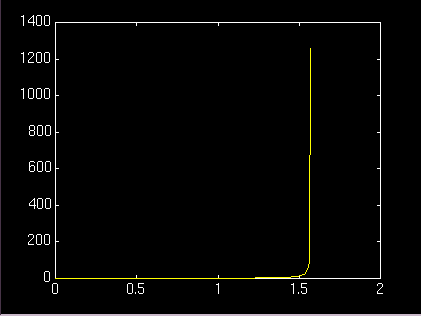
do not produce a very satisfactory result because the automatic scaling of the y-axis is based onx = 0:.01:pi/2;plot(x,tan(x))
ymax = tan(1.57), which is well over 1000.
If the statement is followed by
axis([0 pi/2 0 10])
a much more satisfactory plot results.
Consider the 10-by-5 matrix Z with elements Z(i,j) = j/i. The simplest way to generate this matrix is with doubly nested for loops:
The matrix ism = 10;n = 5;for i = 1:mfor j = 1:nZ(i,j) = j/i;endend
To display this in matrix coordinates, enterZ =1.00 2.00 3.00 4.00 5.000.50 1.00 1.50 2.00 2.500.33 0.67 1.00 1.33 1.67...0.11 0.22 0.33 0.44 0.560.10 0.20 0.30 0.40 0.50
mesh(Z), axis ij
which producesThe plot shows ten rows and five columns. The first element
Z(1,1) = 1.0
is at the upper left; the largest element
Z(1,5) = 5.0
is at the upper right; and the values increase linearly with the column index, j.
On the other hand, consider the function z = f(x,y) = x/y in Cartesian coordinates. This can be evaluated on a grid covering the rectangular region 0 <= x <= 1, 0 <= y <= 2 with
The vectorsm = 10;n = 5;x = (1:n)/n;y = 2*(1:m)'/m;[X,Y] = meshgrid(x,y);Z = X ./ Y;
x and y are
x = [0.20 0.40 0.60 0.80 1.00]
and
y = [0.20 0.40 0.60 ... 1.80 2.00]'
Moreover, the example is arranged so that the 10-by-5 array Z is the same as the one given above.Since this is an example in Cartesian coordinates, enter
mesh(x,y,Z)
which producesNow, even though the matrix is the same, the default Cartesian coordinate system puts the origin at the lower left and the maximum value at the lower right. Moreover, by supplying values for the x- and y- coordinates, different labeling on the axes is obtained.
axis sets the axes object properties XLim, YLim, ZLim, XLimMode, YLimMode, ZLimMode, YDir, and Position.
axes, get, set, subplot
All the properties of axes objects.(c) Copyright 1994 by The MathWorks, Inc.