Dealing with nonlinearity in a system is not an easy task. The difficulty in linearizing a nonlinear system increases with the amount of nonlinearity. In other words, systems described by higher order polynomials are more difficult to linearize than systems which can be represented by lower order polynomials.
The format for linmod is:
[A,B,C,D] = linmod('sfun',x,u,pert,xpert,upert,P1,P2...)
Only the first two inputs above are required. Additional inputs are optional, and should be used if the default values are not satisfactory.When linmod is called upon to perform the linearization, the following happens. Assume we choose default values of zero for both x, the state vector, and the input, u.
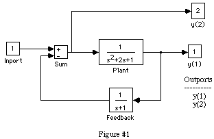
Both Inports and Outports are required, as illustrated in Figure #1, to obtain a linearized model. For multi-input, multi-output models (MIMO), these ports are used to determine about which input/output pair the system is to be linearized. SIMULINK uses the inport as the input to the system. This input u can also be passed in as an optional parameter if the default input does not work well. To solve for the A matrix, this input u is set to the specified value and the states are perturbed about the operating point. For the B, C, and D matrices, the states are set to the operating point, and the input is perturbed. These perturbations are used to determine the rate of change in the state derivatives and outputs (Jacobian).
There are several reasons why linmod (or dlinmod) may not generate a useful linear approximation to the system. One possibility is that the defaults used are not good choices. Many real-world systems do not operate around a state of zero. They need time to reach a viable operating point. Using default values of zero may lead to errors such as "divide by zero" when trying to extract the linear model. This indicates that the operating point being used is not well suited for the system being linearized. To accomplish this task in a simulation, the simulation should be run until a reasonable operating point is reached. At this point, the states x can be output from the simulation and used as the operating point in linmod. The same is true for the input u. Zero is not always the best choice.
Using a Signal Generator or some other input may have a profound effect on the linear approximation. As Inports are required for linearization, other inputs can be used in conjunction with a Sum block. During the linearization process, t remains a constant value of zero. Therefore, the value of the input signal at t = 0 is taken as the input value. Hence, if the input is a unit step function, the value of the step is one at t = 0 and remains this value until the linearization process is complete.
Another common problem which may arise is related to the trade-off between round-off error and truncation error. The numerical algorithms on which linmod is based assume that the system nonlinearities are differentiable. This means they possess a Taylor series expansion. The derivative of a function f(x) at a point x0 can be estimated by computing a finite central difference:
Df(d) = [f(x0 + d) - f(x0 - d)] / 2d (1)provided that the derivative at x0 exists. d represents the perturbation level in the above expression. Complete accuracy would require the perturbation to be infinitesimal and the number of significant figures in the function evaluations to be infinite.
In theory, any error incurred in using (1) is an indication of the curvature of the nonlinearity. If the nonlinear function can be represented by a Taylor-series expansion, the accuracy of (1) depends on how dominant the constant, linear, and quadratic terms are in relation to the higher order terms of the expansion. The expression (1) yields an exact result only for quadratic functions. Errors arise due to the truncation of the higher order terms present in the Taylor series expansion. Such errors are thus called truncation error. Since truncation error increases with perturbation size, the obvious remedy would seem to be to use the smallest perturbation possible.
Alternatively, another source of error lies in the fact that computers have limited precision. Specifying arbitrarily small perturbation levels generally does not work, as the quantities f(x + d),and f(x - d) become nearly equal. When this happens, the central difference loses accuracy; results become dominated by round-off error. Choosing the proper perturbation level is dependent on the situation. Double precision calculations eliminate many, but not all, of these problems. Highly curved nonlinearities or an unfortunate choice of units can still make round-off error a problem.
The linearization algorithm on which linmod is based computes one estimate based on perturbation d, denoted by Df(d), and another estimate based on the perturbation 2d, denoted by Df(2d). It then compares these values for error control to determine an optimal value of d, and returns a weighted combination of the central difference estimate for that optimal d.
Df(d) = [4Df(d) - Df(2d)]/3 (2)The linmod2 function, which uses a slightly different algorithm than linmod, tries to balance the trade-off between round-off error (caused by small perturbations due to finite precision mathematics), and truncation error (caused by large perturbation levels, which invalidate the piecewise linear approximation).
The optional arguments in linmod can be used to specify the perturbation levels for each state and input combination. Obtaining the best model means careful selection of both input and state variable values as well as perturbation levels. How well the linearized model performs can best be examined by comparing the linear model behavior to that of the original nonlinear model.
References:
[1] J.H. Taylor and A.J. Antoniotti, "Linearization Algorithm for ComputerAided Control Engineering". Presented at the 1992 IEEE Symposium on Computer Aided Control System Design, Napa, CA, March 17-19, 1992.
(c) Copyright 1994 by The MathWorks, Inc.