
[t,x] = ode23('xprime',t0,tf,x0)[t,x] = ode23('xprime',t0,tf,x0,tol,trace)[t,x] = ode45('xprime',t0,tf,x0)[t,x] = ode45('xprime',t0,tf,x0,tol,trace)
ode23 and ode45 are functions for the numerical solution of ordinary differential equations. They can solve simple differential equations or simulate complex dynamical systems.A system of nonlinear differential equations can always be expressed as a set of first order differential equations:
where t is (usually) time, x is the state vector, and f is a function that returns the state derivatives as a function of t and x.
ode23 integrates a system of ordinary differential equations using second and third order Runge-Kutta formulas. ode45 uses fourth and fifth order formulas.
The input arguments to ode23 and ode45 are
-------------------------------------------------------------------xprimeA string variable with the name of the M-file that defines the differential equations to be integrated. The function needs to compute the state derivative vector, given the cur rent time and state vector. It must take two input argu ments, scalart(time) and column vectorx(state), and return output argumentxdot, a column vector of state de rivatives: -------------------------------------------------------------------

-------------------------------------------------------------------t0The starting time for the integration (initial value of t).tfThe ending time for the integration (final value of t).x0A column vector of initial conditions.tolOptional - the desired accuracy of the solution. The default value is 1.e-3 forode23, 1.e-6 forode45.traceOptional - flag to print intermediate results. The default value is 0 (don't trace). -------------------------------------------------------------------
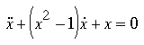
You can rewrite this as a system of coupled first order differential equations:
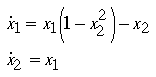
The first step towards simulating this system is to create a function M-file containing these differential equations. Call it vdpol.m:
Note thatfunction xdot = vdpol(t,x)xdot = [x(1).*(1-x(2).^2)-x(2); x(1)]
ode23 requires this function to accept two inputs, t and x, although the function does not use the t input in this case.
To simulate the differential equation defined in vdpol over the interval 0 <= t <= 20, invoke ode23:
The general equations for a dynamical system are sometimes written ast0 = 0; tf = 20;x0 = [0 0.25]'; % Initial conditions[t,x] = ode23('vdpol',t0,tf,x0);plot(t,x)
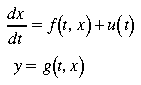
where u is a time dependent vector of external inputs and y is a vector of final measured outputs of the system. Simulation of equations of this form are accomplished in the current framework by recognizing that u(t) can be formed within the xdot function, possibly using a global variable to hold a table of input values, and that y = g(x,t) is simply a final function application to the simulation results.
ode23 and ode45 are M-files that implement algorithms from [1]. On many systems, MEX-file versions are provided for speed.
ode23 and ode45 are automatic step-size Runge-Kutta-Fehlberg integration methods. ode23 uses a simple second and third order pair of formulas for medium accuracy and ode45 uses a fourth and fifth order pair for higher accuracy.
Automatic step-size Runge-Kutta algorithms take larger steps where the solution is more slowly changing. Since ode45 uses higher order formulas, it usually takes fewer integration steps and gives a solution more rapidly. Interpolation (using interp1) can be used to give a smoother time history plot.
ode23 or ode45 cannot perform the integration over the full time range requested, it displays the message
Singularitylikely.
odedemo,SIMULINK


(c) Copyright 1994 by The MathWorks, Inc.