GRID OPERATIONS

Our forestry data is stored in an ASCII file. How do we get it into ARC-INFO and use it with the rest of the data ? Well since the rest of the data is in vector format (arcs and polygons) it would be useful to have the forestry data in that format as well. To start with we must import the data into ARC-INFO. Since the data is set up to be imported as a grid we will do that first. We will use the asciigrid command.

Step 6a : Importing ASCII data into a grid

At the ARC prompt type :

Arc: usage asciigrid
Usage: ASCIIGRID <in_ascii_file> <out_grid> {INT | FLOAT}

Arc: asciigrid forest.dat forestgrid int

Look at the grid you have just created. In ARCPLOT type :


Arcplot: clear        
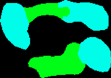
Arcplot: gridpaint forestgrid

Figure 28: gridpaint forestgrid

The green areas are PINE and the pale blue areas are OAK. Now convert this to a polygon coverage, so we can use it with the rest of our data. We will use the gridpoly command.

Step 6b : Converting a grid to a polygon coverage.

In ARC type:

Arc: usage gridpoly

Usage: GRIDPOLY   {weed_tolerance}

Arc: gridpoly forestgrid forestpoly

Converting GRID forestgrid to Coverage forestpoly
 Creating labels...
 Creating forestpoly.PAT...
Arc:

Lets see what information is held in this file (forestpoly.PAT). At the ARC prompt type :


Arc: items forestpoly.pat

COLUMN 	ITEM-NAME		WIDTH	OUTPUT	TYPE	N.DEC 
1  		AREA			4	12	F	3                   
5		PERIMETER		4       12	F	3
9		FORESTPOLY#	        4        5	B	-
13		FORESTPOLY-ID	        4     	 5	B	-
17		GRID-CODE		4     	 8	B	-                        
Arc: 

Arc: list forestpoly.pat
Record	PERIMETER FORESTPOLY# FORESTPOLY-ID GRID-CODE
     1	460000.000     1           0            -9999
     2 	133000.000     2           1                5
     3	107000.000     3           2               10
     4	113999.992     4           3                5
     5	99000.008      5           4                5
     6	139000.000     6           5               10
Arc:

We can see that item GRID-CODE holds the information on tree type - 5 = OAK and 10 = PINE.

Display the polygon file in ARCPLOT.

Arcplot: clear    
Arcplot: polygonshades forestpoly grid-code

Figure 29: Forest polygons.

It should look similar to the image you saw using the gridpaint command except the colors may have changed.

We can overlay this with our current solution coverage to get our flogging areas. To do this we will use the identity command. We will do this next.

go on .

go back

go home