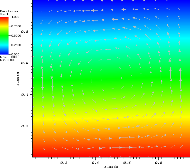
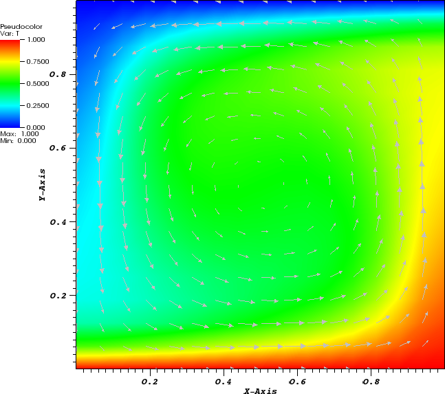
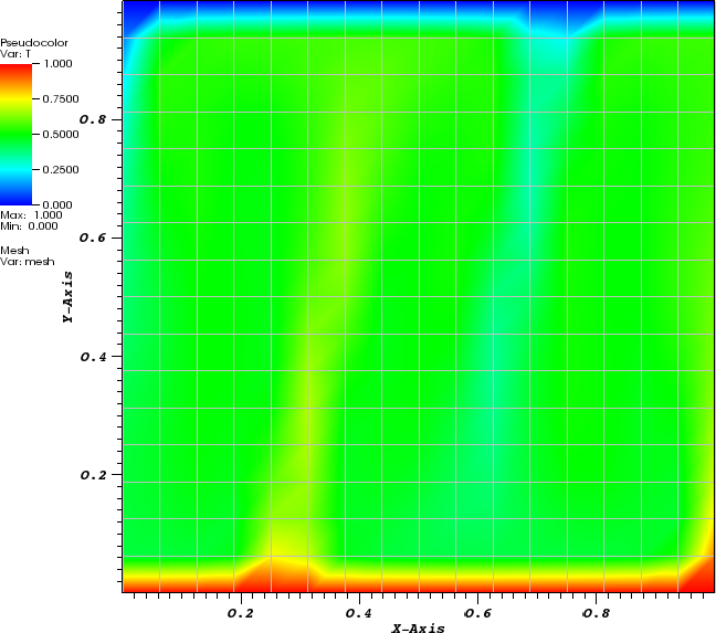
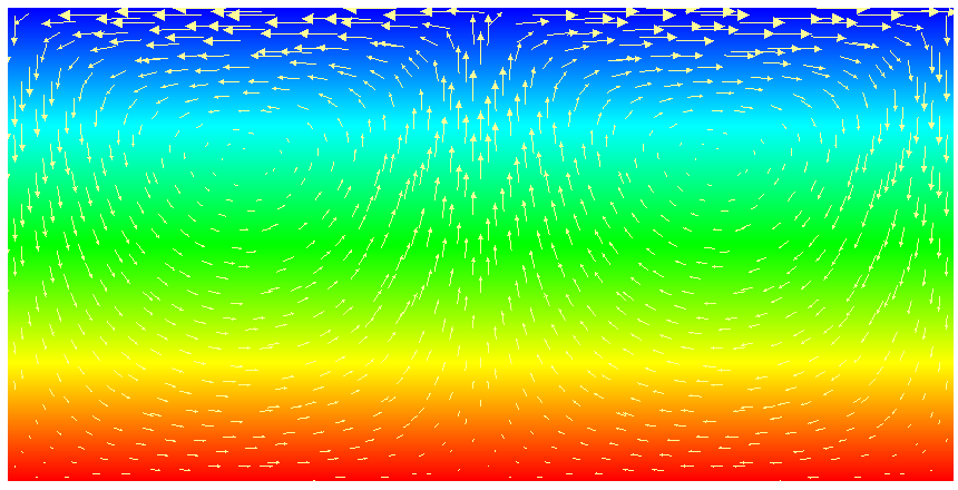
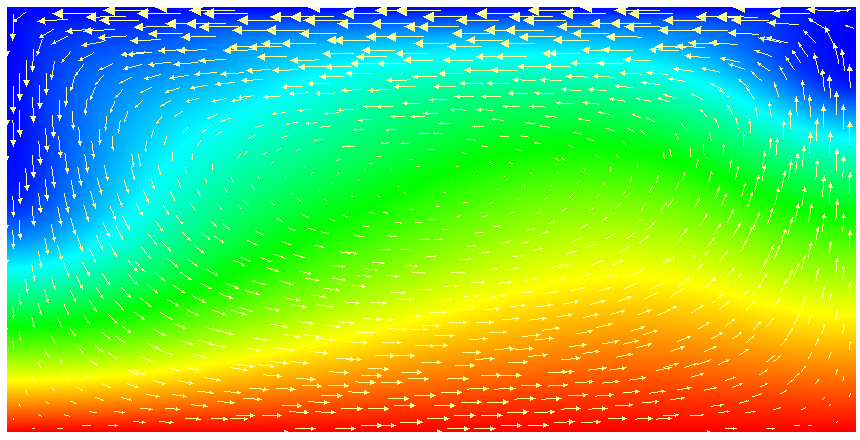
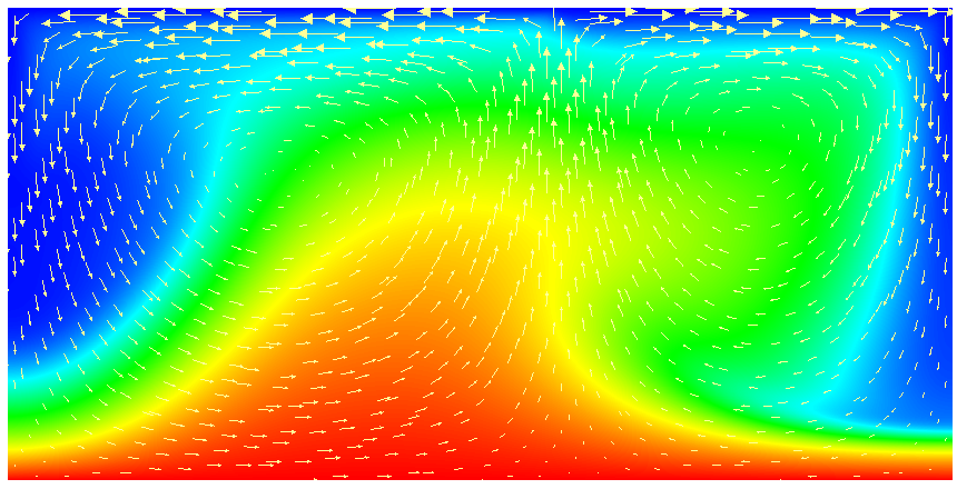
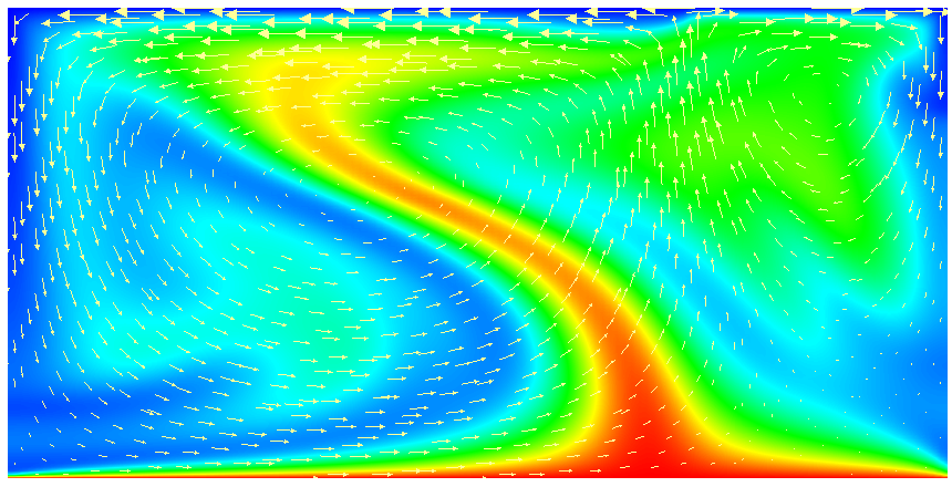
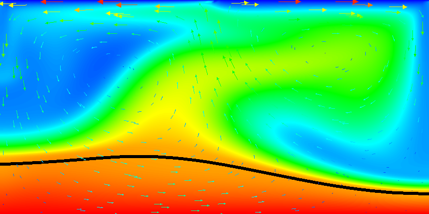
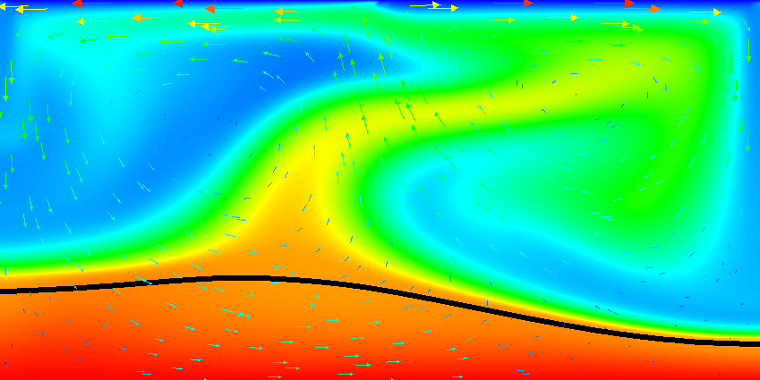
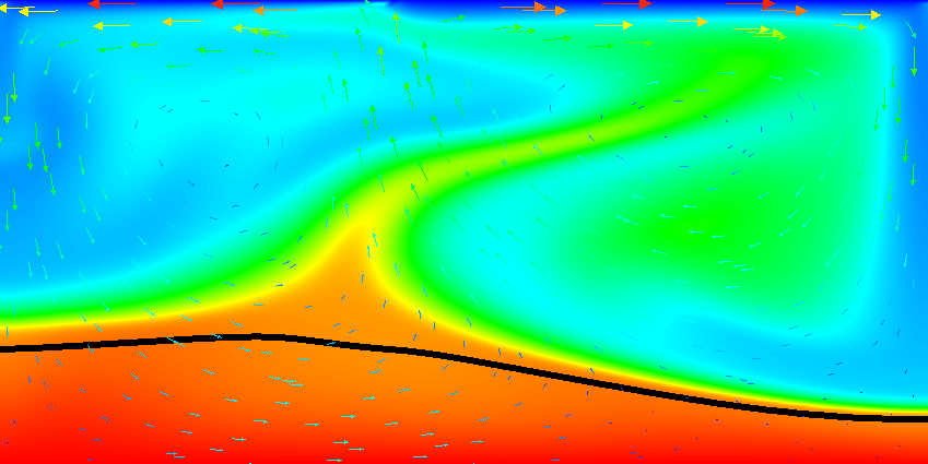
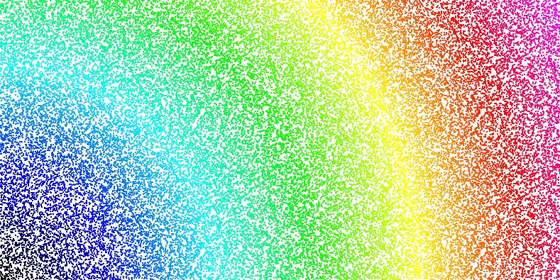
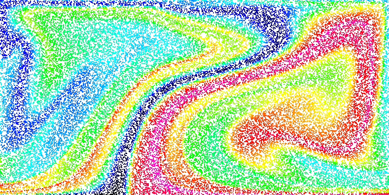
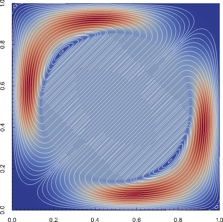
Figure 7: Convection in a box: Initial temperature and velocity field (left) and final state (right).
In this first example, let us consider a simple situation: a 2d box of dimensions that is heated from below, insulated at the left and right, and cooled from the top. We will also consider the simplest model, the incompressible Boussinesq approximation with constant coefficients , for this testcase. Furthermore, we assume that the medium expands linearly with temperature. This leads to the following set of equations:
It is well known that we can non-dimensionalize this set of equations by introducing the Rayleigh number , where is the height of the box, is the thermal diffusivity and is the temperature difference between top and bottom of the box. Formally, we can obtain the non-dimensionalized equations by using the above form and setting coefficients in the following way:
where is the gravity vector in negative -direction. We will see all of these values again in the input file discussed below. One point to note is that for the Boussinesq approximation, as described above, the density in the temperature equation is chosen as the reference density rather than the full density as we see it in the buoyancy term on the right hand side of the momentum equation. As ASPECT is able to handle different approximations of the equations (see Section 2.10), we also have to specify in the input file that we want to use the Boussinesq approximation. The problem is completed by stating the velocity boundary conditions: tangential flow along all four of the boundaries of the box.
This situation describes a well-known benchmark problem for which a lot is known and against which we can compare our results. For example, the following is well understood:
On the other hand, if the Rayleigh number becomes even larger, a series of period doublings starts that makes the system become more and more unstable. We will investigate some of this behavior at the end of this section.
With this said, let us consider how to represent this situation in practice.
The input file. The verbal description of this problem can be translated into an ASPECT input file in the following way (see Section A for a description of all of the parameters that appear in the following input file, and the indices at the end of this manual if you want to find a particular parameter; you can find the input file to run this cookbook example in cookbooks/convection-_box.prm):
Running the program. When you run this program for the first time, you are probably still running ASPECT in debug mode (see Section 4.3) and you will get output like the following:
If you’ve read up on the difference between debug and optimized mode (and you should before you switch!) then consider disabling debug mode. If you run the program again, every number should look exactly the same (and it does, in fact, as I am writing this) except for the timing information printed every hundred time steps and at the end of the program:
In other words, the program ran more than 2 times faster than before. Not all operations became faster to the same degree: assembly, for example, is an area that traverses a lot of code both in ASPECT and in deal.II and so encounters a lot of verification code in debug mode. On the other hand, solving linear systems primarily requires lots of matrix vector operations. Overall, the fact that in this example, assembling linear systems and preconditioners takes so much time compared to actually solving them is primarily a reflection of how simple the problem is that we solve in this example. This can also be seen in the fact that the number of iterations necessary to solve the Stokes and temperature equations is so low. For more complex problems with non-constant coefficients such as the viscosity, as well as in 3d, we have to spend much more work solving linear systems whereas the effort to assemble linear systems remains the same.
Visualizing results. Having run the program, we now want to visualize the numerical results we got. ASPECT can generate graphical output in formats understood by pretty much any visualization program (see the parameters described in Section ??) but we will here follow the discussion in Section 4.4 and use the default VTU output format to visualize using the Visit program.
In the parameter file we have specified that graphical output should be generated every 0.01 time units. Looking through these output files (which can be found in the folder output-convection-box, as specified in the input file), we find that the flow and temperature fields quickly converge to a stationary state. Fig. 7 shows the initial and final states of this simulation.
There are many other things we can learn from the output files generated by ASPECT, specifically from the statistics file that contains information collected at every time step and that has been discussed in Section 4.4.2. In particular, in our input file, we have selected that we would like to compute velocity, temperature, and heat flux statistics. These statistics, among others, are listed in the statistics file whose head looks like this for the current input file:
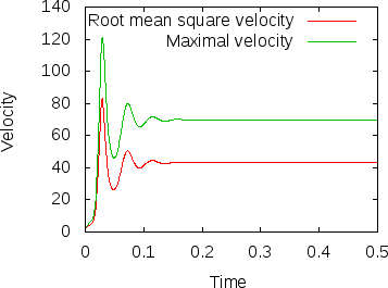
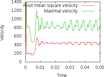
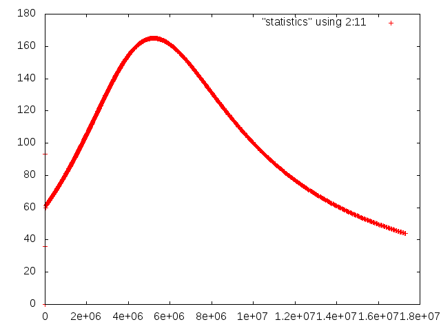
Fig. 8 shows the results of visualizing the data that can be found in columns 2 (the time) plotted against columns 11 and 12 (root mean square and maximal velocities). Plots of this kind can be generated with Gnuplot by typing (see Section 4.4.2 for a more thorough discussion):
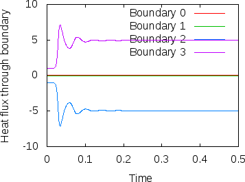
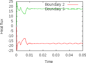
Fig. 8 shows clearly that the simulation enters a steady state after about and then changes very little. This can also be observed using the graphical output files from which we have generated Fig. 7. One can look further into this data to find that the flux through the top and bottom boundaries is not exactly the same (up to the obvious difference in sign, given that at the bottom boundary heat flows into the domain and at the top boundary out of it) at the beginning of the simulation until the fluid has attained its equilibrium. However, after , the fluxes differ by only , i.e., by less than 0.001% of their magnitude.19 The flux we get at the last time step, 4.787, is less than 2% away from the value reported in [BBC89] (4.88) although we compute on a mesh and the values reported by Blankenbach are extrapolated from meshes of size up to . This shows the accuracy that can be obtained using a higher order finite element. Secondly, the fluxes through the left and right boundary are not exactly zero but small. Of course, we have prescribed boundary conditions of the form along these boundaries, but this is subject to discretization errors. It is easy to verify that the heat flux through these two boundaries disappears as we refine the mesh further.
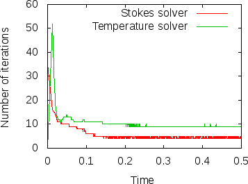
Furthermore, ASPECT automatically also collects statistics about many of its internal workings. Fig. 9 shows the number of iterations required to solve the Stokes and temperature linear systems in each time step. It is easy to see that these are more difficult to solve in the beginning when the solution still changes significant from time step to time step. However, after some time, the solution remains mostly the same and solvers then only need 9 or 10 iterations for the temperature equation and 4 or 5 iterations for the Stokes equations because the starting guess for the linear solver – the previous time step’s solution – is already pretty good. If you look at any of the more complex cookbooks, you will find that one needs many more iterations to solve these equations.
Play time 1: Different Rayleigh numbers. After showing you results for the input file as it can be found in cookbooks/convection-_box.prm, let us end this section with a few ideas on how to play with it and what to explore. The first direction one could take this example is certainly to consider different Rayleigh numbers. As mentioned above, for the value for which the results above have been produced, one gets a stable convection pattern. On the other hand, for values , any movement of the fluid dies down exponentially and we end up with a situation where the fluid doesn’t move and heat is transported from the bottom to the top only through heat conduction. This can be explained by considering that the Rayleigh number in a box of unit extent is defined as . A small Rayleigh number means that the viscosity is too large (i.e., the buoyancy given by the product of the magnitude of gravity times the density anomalies caused by temperature – – is not strong enough to overcome friction forces within the fluid).
On the other hand, if the Rayleigh number is large (i.e., the viscosity is small or the buoyancy large) then the fluid develops an unsteady convection period. As we consider fluids with larger and larger , this pattern goes through a sequence of period-doubling events until flow finally becomes chaotic. The structures of the flow pattern also become smaller and smaller.

We illustrate these situations in Fig.s 10 and 11. The first shows the temperature field at the end of a simulation for (below ) and at . Obviously, for the right picture, the mesh is not fine enough to accurately resolve the features of the flow field and we would have to refine it more. The second of the figures shows the velocity and heatflux statistics for the computation with ; it is obvious here that the flow no longer settles into a steady state but has a periodic behavior. This can also be seen by looking at movies of the solution.
To generate these results, remember that we have chosen in our input file. In other words, changing the input file to contain the parameter setting
will achieve the desired effect of computing with .
Play time 2: Thinking about finer meshes. In our computations for we used a mesh and obtained a value for the heat flux that differed from the generally accepted value from Blankenbach et al. [BBC89] by less than 2%. However, it may be interesting to think about computing even more accurately. This is easily done by using a finer mesh, for example. In the parameter file above, we have chosen the mesh setting as follows:
We start out with a box geometry consisting of a single cell that is refined four times. Each time we split each cell into its 4 children, obtaining the mesh already mentioned. The other settings indicate that we do not want to refine the mesh adaptively at all in the first time step, and a setting of zero for the last parameter means that we also never want to adapt the mesh again at a later time. Let us stick with the never-changing, globally refined mesh for now (we will come back to adaptive mesh refinement again at a later time) and only vary the initial global refinement. In particular, we could choose the parameter Initial global refinement to be 5, 6, or even larger. This will get us closer to the exact solution albeit at the expense of a significantly increased computational time.
A better strategy is to realize that for , the flow enters a steady state after settling in during the first part of the simulation (see, for example, the graphs in Fig. 8). Since we are not particularly interested in this initial transient process, there is really no reason to spend CPU time using a fine mesh and correspondingly small time steps during this part of the simulation (remember that each refinement results in four times as many cells in 2d and a time step half as long, making reaching a particular time at least 8 times as expensive, assuming that all solvers in ASPECT scale perfectly with the number of cells). Rather, we can use a parameter in the ASPECT input file that let’s us increase the mesh resolution at later times. To this end, let us use the following snippet for the input file:
What this does is the following: We start with an mesh (3 times globally refined) but then at times and we refine the mesh using the default refinement indicator (which one this is is not important because of the next statement). Each time, we refine, we refine a fraction 1.0 of the cells, i.e., all cells and we coarsen a fraction of 0.0 of the cells, i.e. no cells at all. In effect, at these additional refinement times, we do another global refinement, bringing us to refinement levels 4, 5 and finally 6.
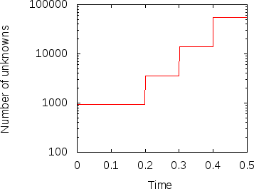
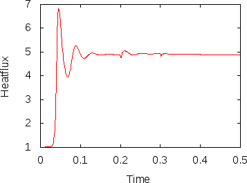
Fig. 12 shows the results. In the left panel, we see how the number of unknowns grows over time (note the logscale for the -axis). The right panel displays the heat flux. The jumps in the number of cells is clearly visible in this picture as well. This may be surprising at first but remember that the mesh is clearly too coarse in the beginning to really resolve the flow and so we should expect that the solution changes significantly if the mesh is refined. This effect becomes smaller with every additional refinement and is barely visible at the last time this happens, indicating that the mesh before this refinement step may already have been fine enough to resolve the majority of the dynamics.
In any case, we can compare the heat fluxes we obtain at the end of these computations: With a globally four times refined mesh, we get a value of 4.787 (an error of approximately 2% against the accepted value from Blankenbach, ). With a globally five times refined mesh we get 4.879, and with a globally six times refined mesh we get 4.89 (an error of almost 0.1%). With the mesh generated using the procedure above we also get 4.89 with the digits printed on the screen20 (also corresponding to an error of almost 0.1%). In other words, our simple procedure of refining the mesh during the simulation run yields the same accuracy as using the mesh that is globally refined in the beginning of the simulation, while needing a much lower compute time.
Play time 3: Changing the finite element in use. Another way to increase the accuracy of a finite element computation is to use a higher polynomial degree for the finite element shape functions. By default, ASPECT uses quadratic shape functions for the velocity and the temperature and linear ones for the pressure. However, this can be changed with a single number in the input file.
Before doing so, let us consider some aspects of such a change. First, looking at the pictures of the solution in Fig. 7, one could surmise that the quadratic elements should be able to resolve the velocity field reasonably well given that it is rather smooth. On the other hand, the temperature field has a boundary layer at the top and bottom. One could conjecture that the temperature polynomial degree is therefore the limiting factor and not the polynomial degree for the flow variables. We will test this conjecture below. Secondly, given the nature of the equations, increasing the polynomial degree of the flow variables increases the cost to solve these equations by a factor of in 2d (you can get this factor by counting the number of degrees of freedom uniquely associated with each cell) but leaves the time step size and the cost of solving the temperature system unchanged. On the other hand, increasing the polynomial degree of the temperature variable from 2 to 3 requires times as many degrees of freedom for the temperature and also requires us to reduce the size of the time step by a factor of . Because solving the temperature system is not a dominant factor in each time step (see the timing results shown at the end of the screen output above), the reduction in time step is the only important factor. Overall, increasing the polynomial degree of the temperature variable turns out to be the cheaper of the two options.
Following these considerations, let us add the following section to the parameter file:
This leaves the velocity and pressure shape functions at quadratic and linear polynomial degree but increases the polynomial degree of the temperature from quadratic to cubic. Using the original, four times globally refined mesh, we then get the following output:
The heat flux through the top and bottom boundaries is now computed as 4.878. Using the five times globally refined mesh, it is 4.8837 (an error of 0.015%). This is 6 times more accurate than the once more globally refined mesh with the original quadratic elements, at a cost significantly smaller. Furthermore, we can of course combine this with the mesh that is gradually refined as simulation time progresses, and we then get a heat flux that is equal to 4.884446, also only 0.01% away from the accepted value!
As a final remark, to test our hypothesis that it was indeed the temperature polynomial degree that was the limiting factor, we can increase the Stokes polynomial degree to 3 while leaving the temperature polynomial degree at 2. A quick computation shows that in that case we get a heat flux of 4.747 – almost the same value as we got initially with the lower order Stokes element. In other words, at least for this testcase, it really was the temperature variable that limits the accuracy.
The world is not two-dimensional. While the previous section introduced a number of the knobs one can play with with ASPECT, things only really become interesting once one goes to 3d. The setup from the previous section is easily adjusted to this and in the following, let us walk through some of the changes we have to consider when going from 2d to 3d. The full input file that contains these modifications and that was used for the simulations we will show subsequently can be found at cookbooks/convection-_box-_3d.prm.
The first set of changes has to do with the geometry: it is three-dimensional, and we will have to address the fact that a box in 3d has 6 sides, not the 4 we had previously. The documentation of the “box” geometry (see Section ??) states that these sides are numbered as follows: “in 3d, boundary indicators 0 through 5 indicate left, right, front, back, bottom and top boundaries.” Recalling that we want tangential flow all around and want to fix the temperature to known values at the bottom and top, the following will make sense:
The next step is to describe the initial conditions. As before, we will use an unstably layered medium but the perturbation now needs to be both in - and -direction
The third issue we need to address is that we can likely not afford a mesh as fine as in 2d. We choose a mesh that is refined 3 times globally at the beginning, then 3 times adaptively, and is then adapted every 15 time steps. We also allow one additional mesh refinement in the first time step following once the initial instability has given way to a more stable pattern:
Finally, as we have seen in the previous section, a computation with does not lead to a simulation that is exactly exciting. Let us choose instead (the mesh chosen above with up to 7 refinement levels after some time is fine enough to resolve this). We can achieve this in the same way as in the previous section by choosing and setting
This has some interesting implications. First, a higher Rayleigh number makes time scales correspondingly smaller; where we generated graphical output only once every 0.01 time units before, we now need to choose the corresponding increment smaller by a factor of 100:
Secondly, a simulation like this – in 3d, with a significant number of cells, and for a significant number of time steps – will likely take a good amount of time. The computations for which we show results below was run using 64 processors by running it using the command mpirun -n 64 ./aspect convection-box-3d.prm. If the machine should crash during such a run, a significant amount of compute time would be lost if we had to run everything from the start. However, we can avoid this by periodically checkpointing the state of the computation:
If the computation does crash (or if a computation runs out of the time limit imposed by a scheduling system), then it can be restarted from such checkpointing files (see the parameter Resume computation in Section ??).
Running with this input file requires a bit of patience21 since the number of degrees of freedom is just so large: it starts with a bit over 330,000…
…but then increases quickly to around 2 million as the solution develops some structure and, after time where we allow for an additional refinement, increases to over 10 million where it then hovers between 8 and 14 million with a maximum of 15,147,534. Clearly, even on a reasonably quick machine, this will take some time: running this on a machine bought in 2011, doing the 10,000 time steps to get to takes approximately 484,000 seconds (about five and a half days).
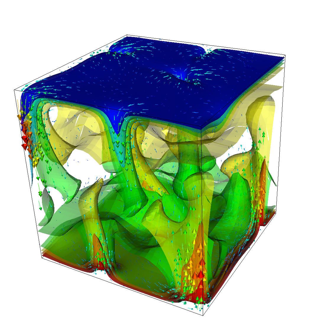
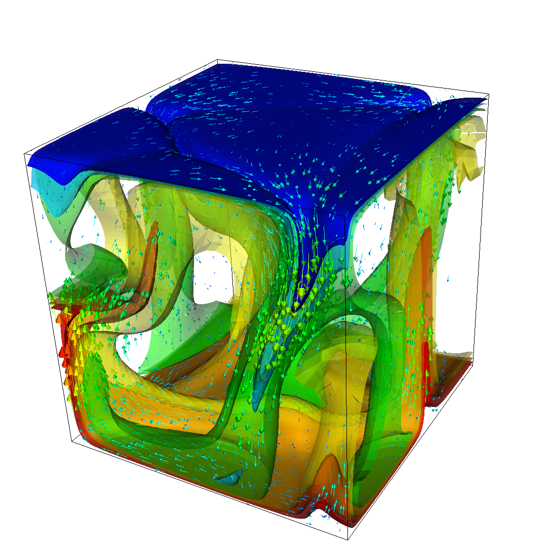
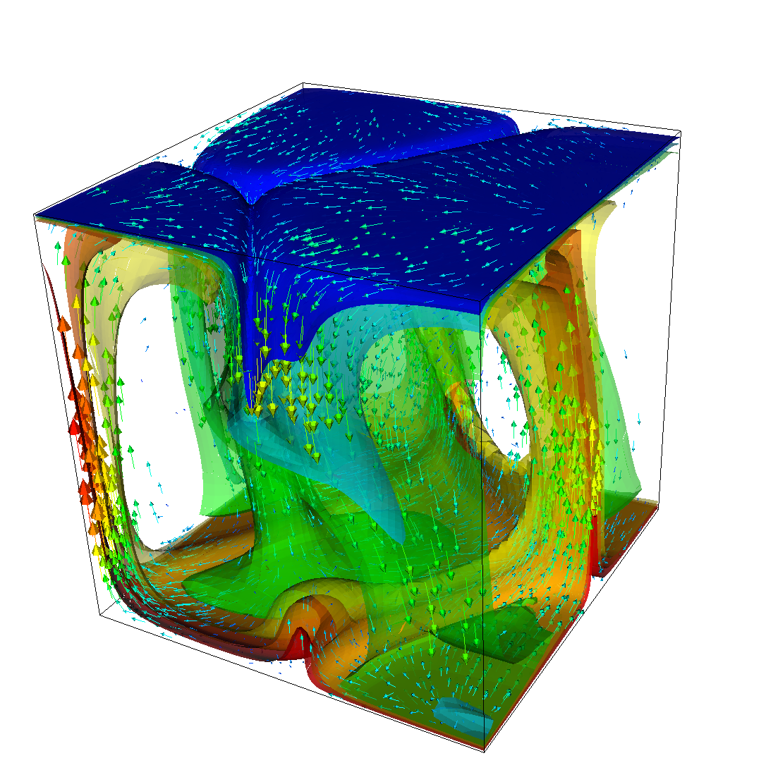
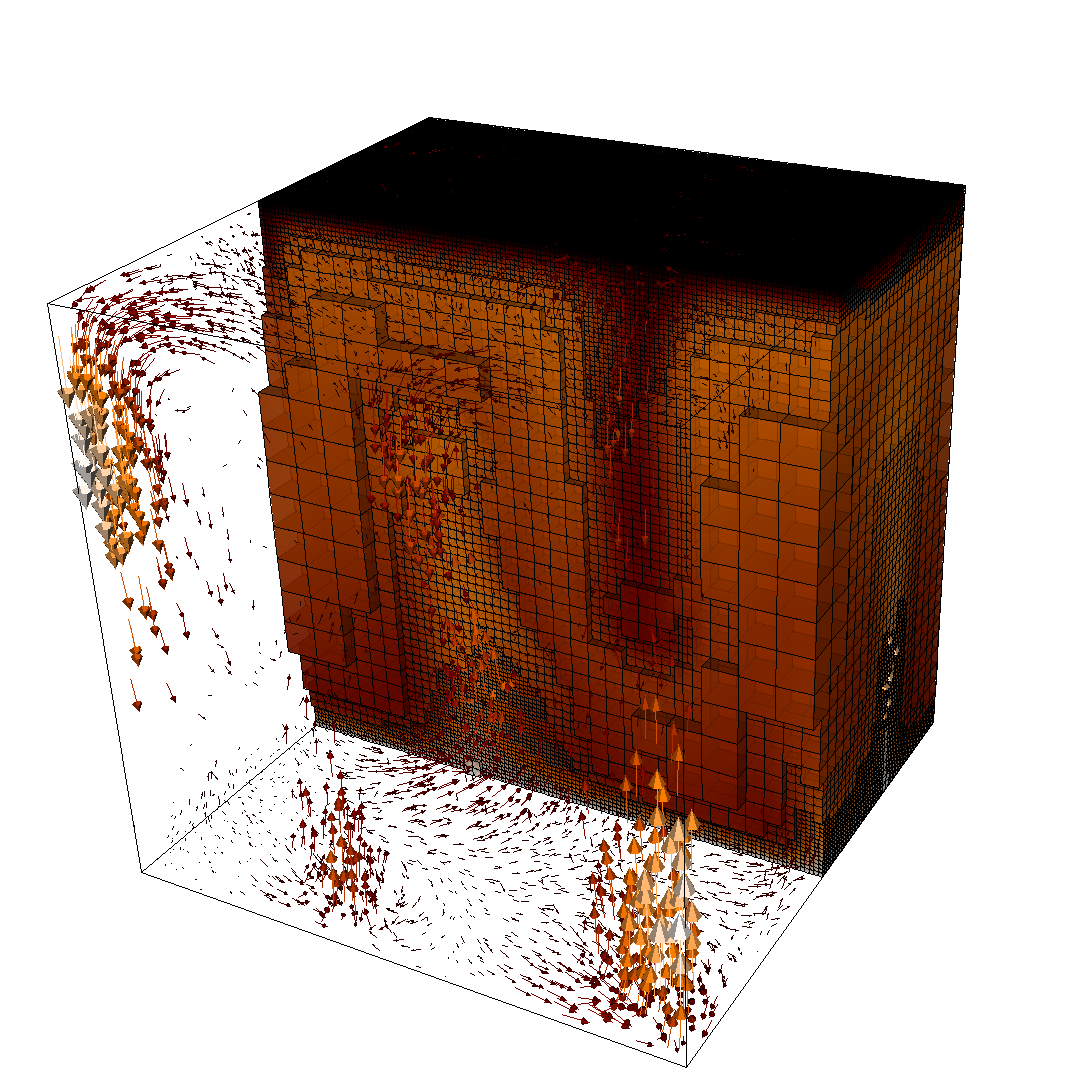
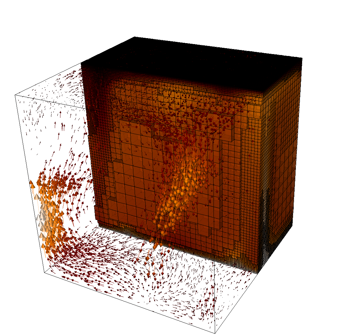
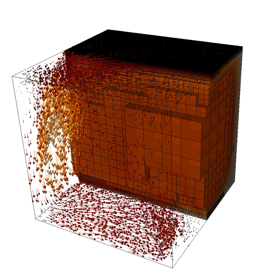
The structure or the solution is easiest to grasp by looking at isosurfaces of the temperature. This is shown in Fig. 13 and you can find a movie of the motion that ensues from the heating at the bottom at http://www.youtube.com/watch?v=_bKqU_P4j48. The simulation uses adaptively changing meshes that are fine in rising plumes and sinking blobs and are coarse where nothing much happens. This is most easily seen in the movie at http://www.youtube.com/watch?v=CzCKYyR-_cmg. Fig. 14 shows some of these meshes, though still pictures do not do the evolving nature of the mesh much justice. The effect of increasing the Rayleigh number is apparent when comparing the size of features with, for example, the picture at the right of Fig. 7. In contrast to that picture, the simulation is also clearly non-stationary.
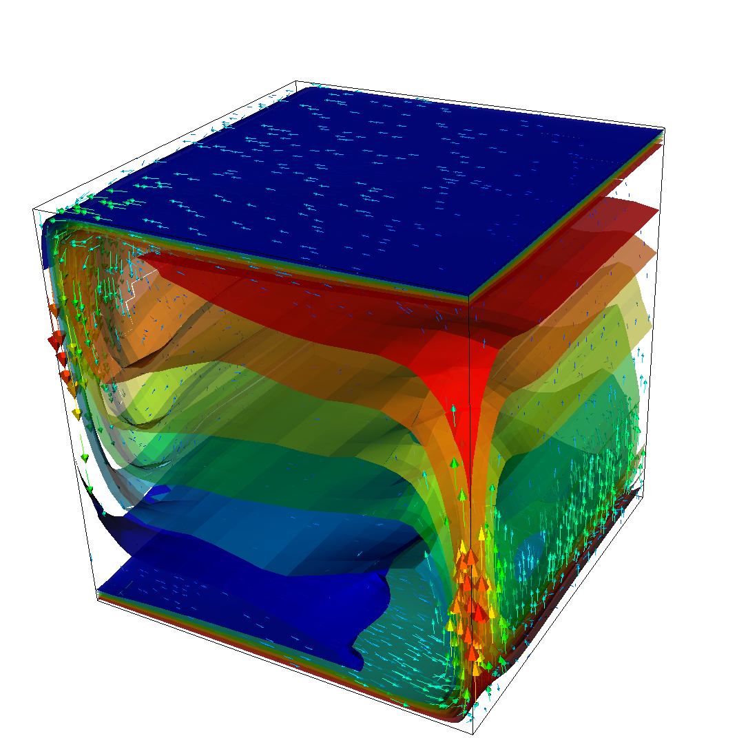
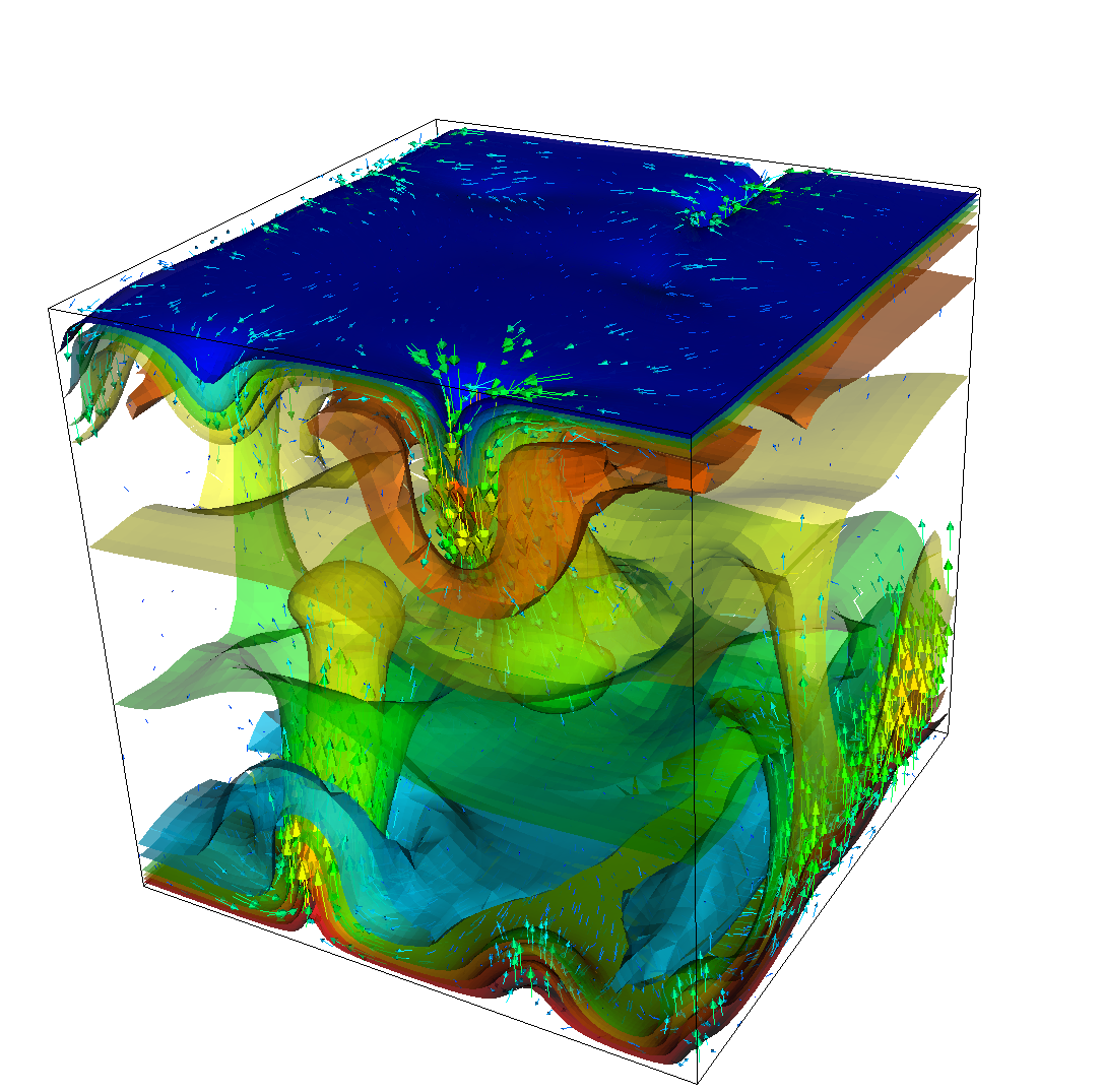
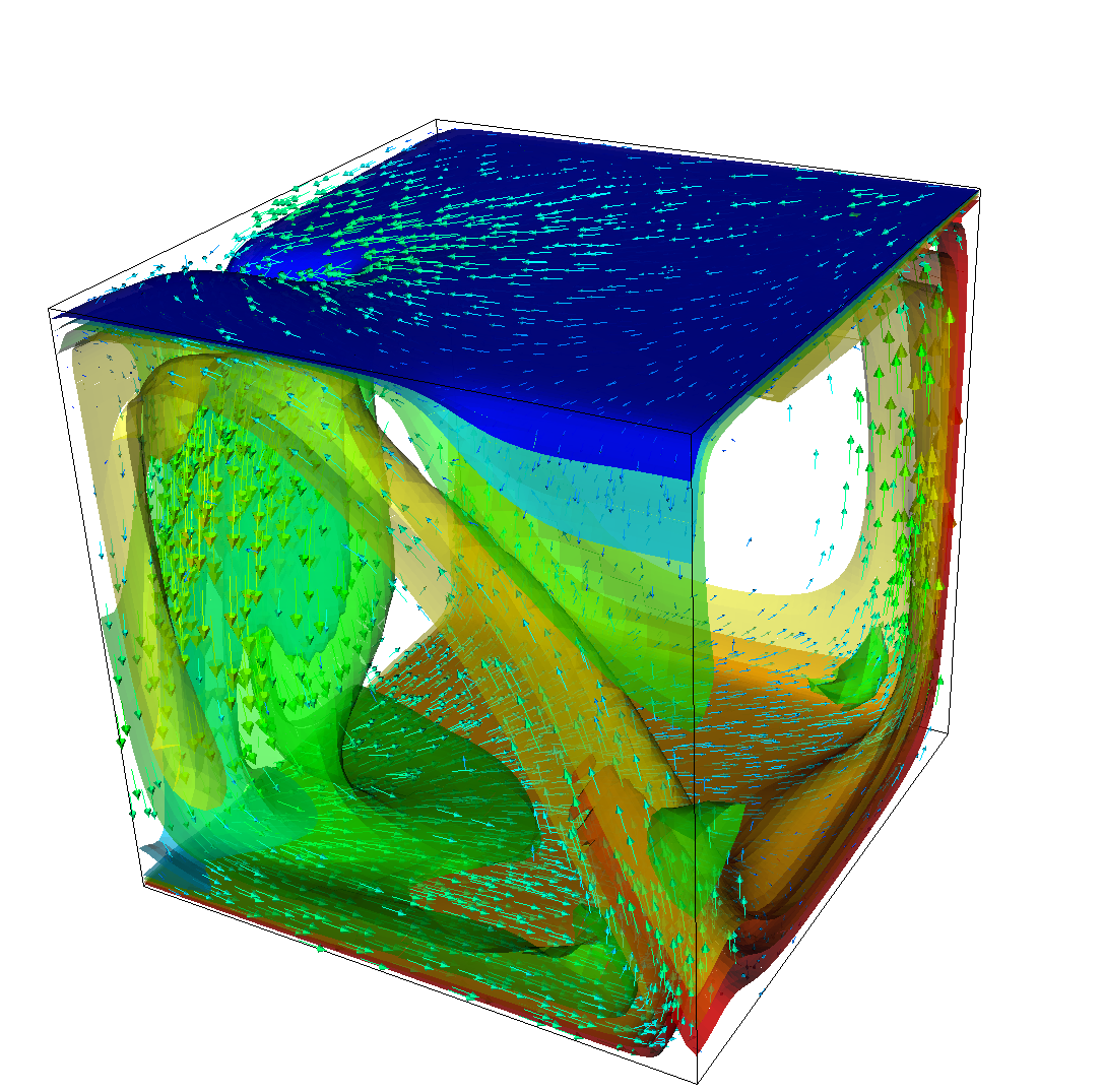
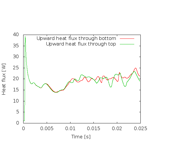
As before, we could analyze all sorts of data from the statistics file but we will leave this to those interested in specific data. Rather, Fig. 15 only shows the upward heat flux through the bottom and top boundaries of the domain as a function of time.22 The figure reinforces a pattern that can also be seen by watching the movie of the temperature field referenced above, namely that the simulation can be subdivided into three distinct phases. The first phase corresponds to the initial overturning of the unstable layering of the temperature field and is associated with a large spike in heat flux as well as large velocities (not shown here). The second phase, until approximately corresponds to a relative lull: some plumes rise up, but not very fast because the medium is now stably layered but not fully mixed. This can be seen in the relatively low heat fluxes, but also in the fact that there are almost horizontal temperature isosurfaces in the second of the pictures in Fig. 13. After that, the general structure of the temperature field is that the interior of the domain is well mixed with a mostly constant average temperature and thin thermal boundary layers at the top and bottom from which plumes rise and sink. In this regime, the average heat flux is larger but also more variable depending on the number of plumes currently active. Many other analyses would be possible by using what is in the statistics file or by enabling additional postprocessors.
A similarly simple setup to the ones considered in the previous subsections is to equip the model we had with a different set of boundary conditions. There, we used slip boundary conditions, i.e., the fluid can flow tangentially along the four sides of our box but this tangential velocity is unspecified. On the other hand, in many situations, one would like to actually prescribe the tangential flow velocity as well. A typical application would be to use boundary conditions at the top that describe experimentally determined velocities of plates. This cookbook shows a simple version of something like this. To make it slightly more interesting, we choose a domain in 2d.
Like for many other things, ASPECT has a set of plugins for prescribed velocity boundary values (see Sections ?? and 6.3.6). These plugins allow one to write sophisticated models for the boundary velocity on parts or all of the boundary, but there is also one simple implementation that just takes a formula for the components of the velocity.
To illustrate this, let us consider the cookbooks/platelike-_boundary.prm input file. It essentially extends the input file considered in the previous example. The part of this file that we are particularly interested in in the current context is the selection of the kind of velocity boundary conditions on the four sides of the box geometry, which we do using a section like this:
We use tangential flow at boundaries named left, right and bottom. Additionally, we specify a comma separated list (here with only a single element) of pairs consisting of the name of a boundary and the name of a prescribed velocity boundary model. Here, we use the function model on the top boundary, which allows us to provide a function-like notation for the components of the velocity vector at the boundary.
The second part we need is that we actually describe the function that sets the velocity. We do this in the subsection Function. The first of these parameters gives names to the components of the position vector (here, we are in 2d and we use and as spatial variable names) and the time. We could have left this entry at its default, x,y,t, but since we often think in terms of “depth” as the vertical direction, let us use z for the second coordinate. In the second parameter we define symbolic constants that can be used in the formula for the velocity that is specified in the last parameter. This formula needs to have as many components as there are space dimensions, separated by semicolons. As stated, this means that we prescribe the (horizontal) -velocity and set the vertical velocity to zero. The horizontal component is here either or , depending on whether we are to the right or the left of the point that is moving back and forth with time once every four time units. The if statement understood by the parser we use for these formulas has the syntax if(condition, value-if-true, value-if-false).
It is in general not possible for ASPECT to verify that a given input is sensible. However, you
will quickly find out if it isn’t: The linear solver for the Stokes equations will simply not converge.
For example, if your function expression in the input file above read
if(x>1+sin(0.5*pi*t), 1, -1); 1
then at the time of writing this you would get the following error message:
*** Timestep 0: t=0 seconds
Solving temperature system... 0 iterations.
Rebuilding Stokes preconditioner...
Solving Stokes system...
…some timing output …
––––––––––––––––––––––––––
Exception on processing:
Iterative method reported convergence failure in step 9539 with residual 6.0552
Aborting!
––––––––––––––––––––––––––
The reason is, of course, that there is no incompressible (divergence free) flow field that allows for a constant vertical outflow component along the top boundary without corresponding inflow anywhere else.
The remainder of the setup is described in the following, complete input file:
This model description yields a setup with a Rayleigh number of 200 (taking into account that the domain has size 2). It would, thus, be dominated by heat conduction rather than convection if the prescribed velocity boundary conditions did not provide a stirring action. Visualizing the results of this simulation23 yields images like the ones shown in Fig. 16.
One frequently wants to track where material goes, either because one simply wants to see where stuff ends up (e.g., to determine if a particular model yields mixing between the lower and upper mantle) or because the material model in fact depends not only pressure, temperature and location but also on the mass fractions of certain chemical or other species. We will refer to the first case as passive and the latter as active to indicate the role of the additional quantities whose distribution we want to track. We refer to the whole process as compositional since we consider quantities that have the flavor of something that denotes the composition of the material at any given point.
There are basically two ways to achieve this: one can advect a set of particles (“tracers”) along with the velocity field, or one can advect along a field. In the first case, where the closest particle came from indicates the value of the concentration at any given position. In the latter case, the concentration(s) at any given position is simply given by the value of the field(s) at this location.
ASPECT implements both strategies, at least to a certain degree. In this cookbook, we will follow the route of advected fields.
The passive case. We will consider the exact same situation as in the previous section but we will ask where the material that started in the bottom 20% of the domain ends up, as well as the material that started in the top 20%. For the moment, let us assume that there is no material between the materials at the bottom, the top, and the middle. The way to describe this situation is to simply add the following block of definitions to the parameter file (you can find the full parameter file in cookbooks/composition-_passive.prm:
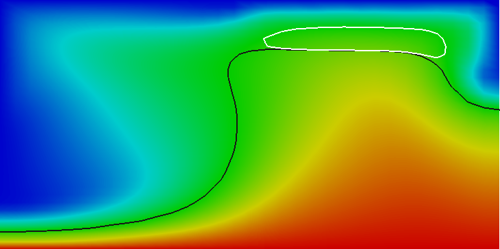
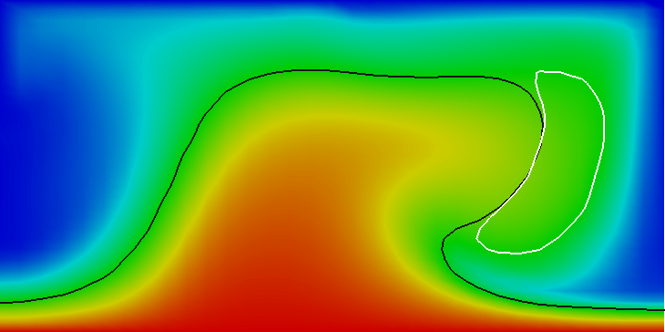
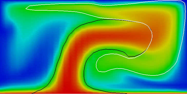
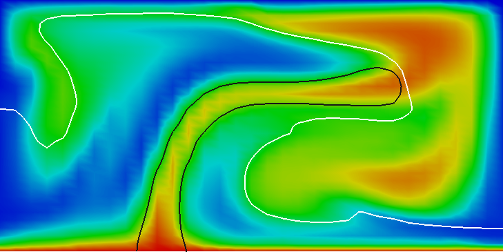
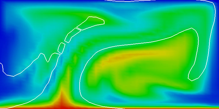
Running this simulation yields results such as the ones shown in Fig. 17 where we show the values of the functions and at various times in the simulation. Because these fields were one only inside the lowermost and uppermost parts of the domain, zero everywhere else, and because they have simply been advected along with the flow field, the places where they are larger than one half indicate where material has been transported to so far.24
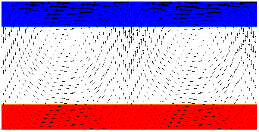
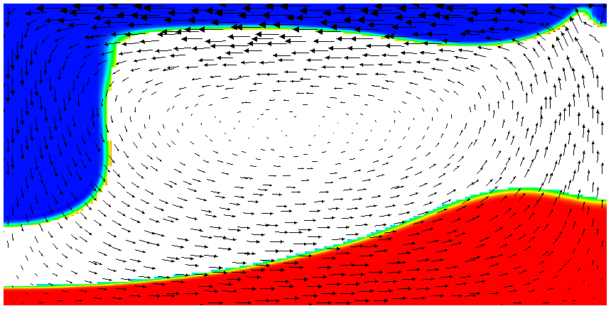
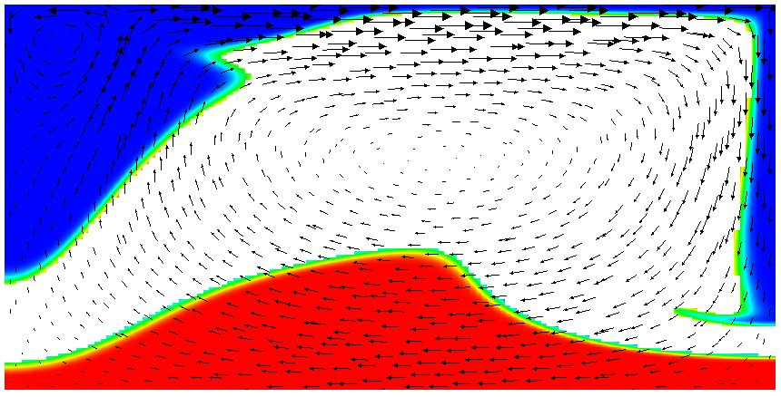
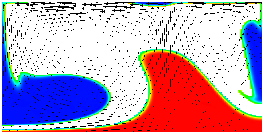
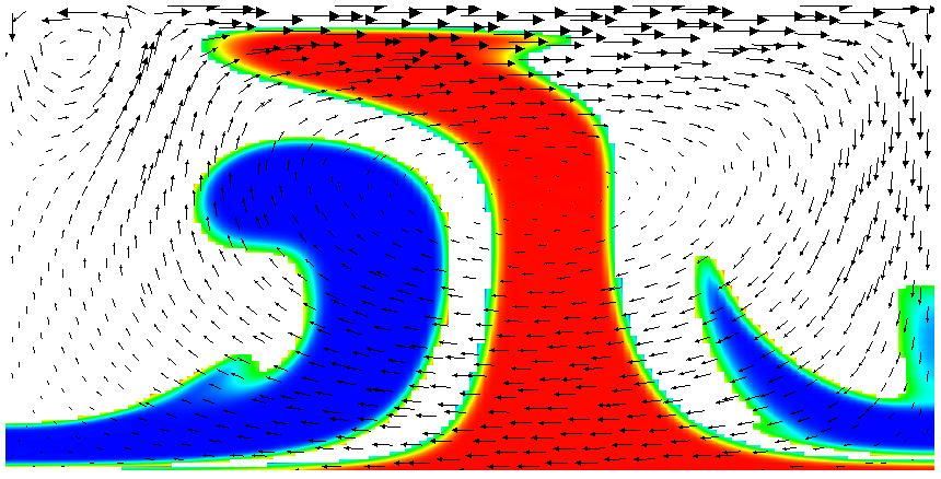
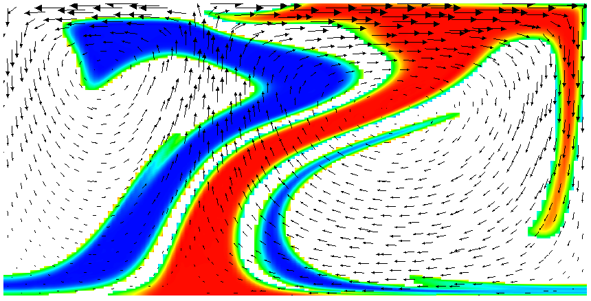
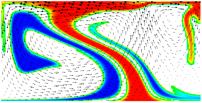
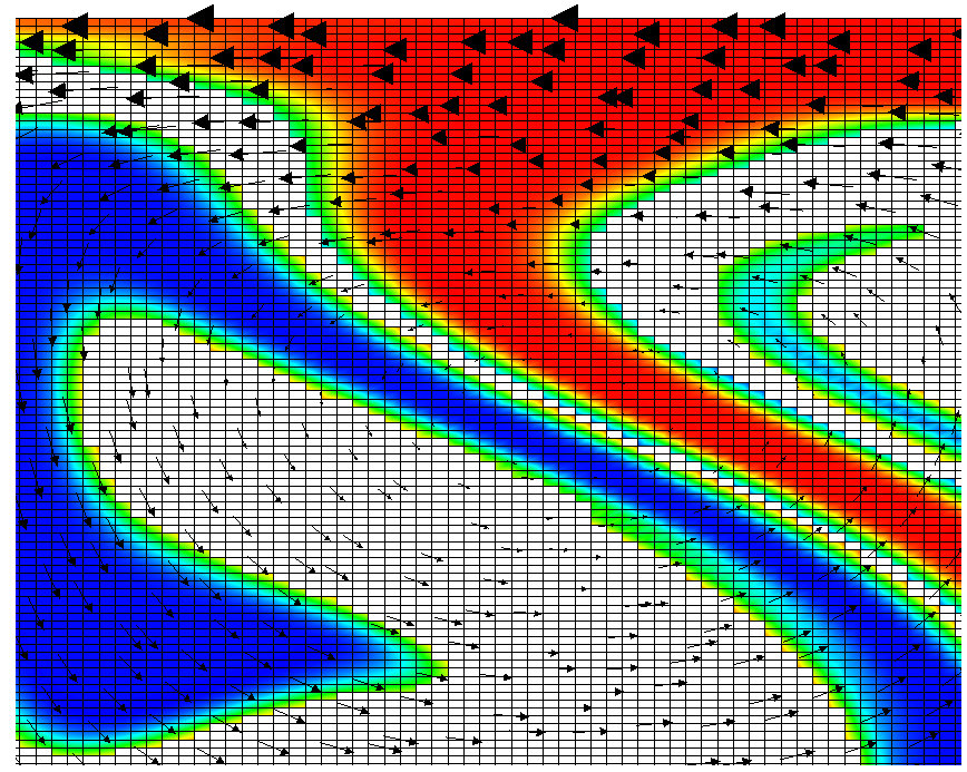
Fig. 17 shows one aspect of compositional fields that occasionally makes them difficult to use for very long time computations. The simulation shown here runs for 20 time units, where every cycle of the spreading center at the top moving left and right takes 4 time units, for a total of 5 such cycles. While this is certainly no short-term simulation, it is obviously visible in the figure that the interface between the materials has diffused over time. Fig. 18 shows a zoom into the center of the domain at the final time of the simulation. The figure only shows values that are larger than 0.5, and it looks like the transition from red or blue to the edge of the shown region is no wider than 3 cells. This means that the computation is not overly diffusive but it is nevertheless true that this method has difficulty following long and thin filaments.25 This is an area in which ASPECT may see improvements in the future.
A different way of looking at the quality of compositional fields as opposed to particles is to ask whether they conserve mass. In the current context, the mass contained in the th compositional field is . This can easily be achieve in the following way, by adding the composition statistics postprocessor:
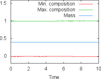
While the scheme we use to advect the compositional fields is not strictly conservative, it is almost perfectly so in practice. For example, in the computations shown in this section (using two additional global mesh refinements over the settings in the parameter file cookbooks/composition-_passive.prm), Fig. 19 shows the maximal and minimal values of the first compositional fields over time, along with the mass (these are all tabulated in columns of the statistics file, see Sections 4.1 and 4.4.2). While the maximum and minimum fluctuate slightly due to the instability of the finite element method in resolving discontinuous functions, the mass appears stable at a value of 0.403646 (the exact value, namely the area that was initially filled by each material, is 0.4; the difference is a result of the fact that we can’t exactly represent the step function on our mesh with the finite element space). In fact, the maximal difference in this value between time steps 1 and 500 is only . In other words, these numbers show that the compositional field approach is almost exactly mass conservative.
The active case. The next step, of course, is to make the flow actually depend on the composition. After all, compositional fields are not only intended to indicate where material come from, but also to indicate the properties of this material. In general, the way to achieve this is to write material models where the density, viscosity, and other parameters depend on the composition, taking into account what the compositional fields actually denote (e.g., if they simply indicate the origin of material, or the concentration of things like olivine, perovskite, …). The construction of material models is discussed in much greater detail in Section 6.3.1; we do not want to revisit this issue here and instead choose – once again – the simplest material model that is implemented in ASPECT: the simple model.
The place where we are going to hook in a compositional dependence is the density. In the simple model, the density is fundamentally described by a material that expands linearly with the temperature; for small density variations, this corresponds to a density model of the form . This is, by virtue of its simplicity, the most often considered density model. But the simple model also has a hook to make the density depend on the first compositional field , yielding a dependence of the form . Here, let us choose . The rest of our model setup will be as in the passive case above. Because the temperature will be between zero and one, the temperature induced density variations will be restricted to 0.01, whereas the density variation by origin of the material is 100. This should make sure that dense material remains at the bottom despite the fact that it is hotter than the surrounding material.26
This setup of the problem can be described using an input file that is almost completely unchanged from the passive case. The only difference is the use of the following section (the complete input file can be found in cookbooks/composition-_active.prm:
To debug the model, we will also want to visualize the density in our graphical output files. This is done using the following addition to the postprocessing section, using the density visualization plugin:
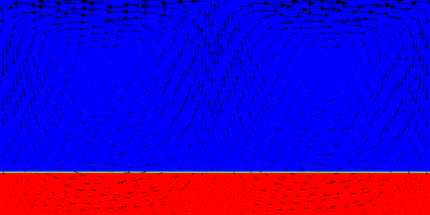
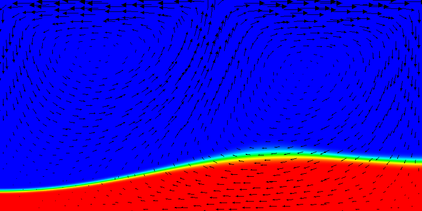
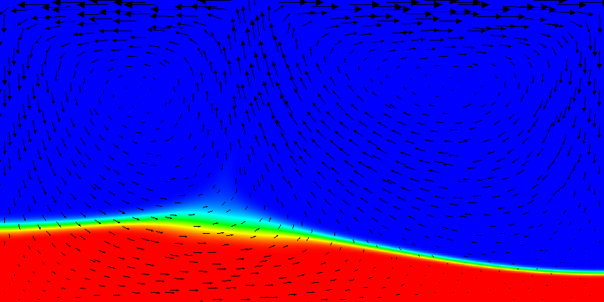

Results of this model are visualized in Fig.s 20 and 21. What is visible is that over the course of the simulation, the material that starts at the bottom of the domain remains there. This can only happen if the circulation is significantly affected by the high density material once the interface starts to become non-horizontal, and this is indeed visible in the velocity vectors. As a second consequence, if the material at the bottom does not move away, then there needs to be a different way for the heat provided at the bottom to get through the bottom layer: either there must be a secondary convection system in the bottom layer, or heat is simply conducted. The pictures in the figure seem to suggest that the latter is the case.
It is easy, using the outline above, to play with the various factors that drive this system, namely:
Using the coefficients involved in these considerations, it is trivially possible to map out the parameter space to find which of these effects is dominant. As mentioned in discussing the values in the input file, what is important is the relative size of these parameters, not the fact that currently the density in the material at the bottom is 100 times larger than in the rest of the domain, an effect that from a physical perspective clearly makes no sense at all.
The active case with reactions. This section was contributed by Juliane Dannberg and René Gaßmöller.
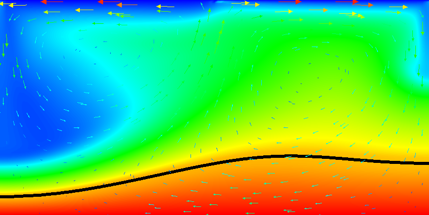
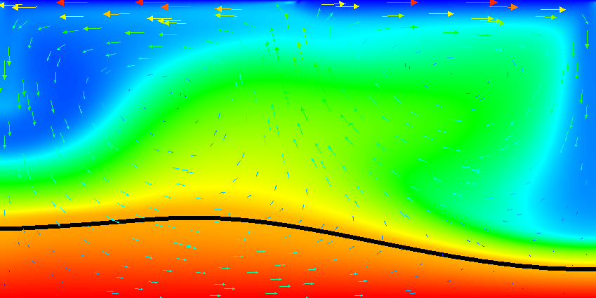
In addition, there are setups where one wants the compositional fields to interact with each other. One example would be material upwelling at a mid-ocean ridge and changing the composition to that of oceanic crust when it reaches a certain depth. In this cookbook, we will describe how this kind of behaviour can be achieved by using the composition reaction function of the material model.
We will consider the exact same setup as in the previous paragraphs, except for the initial conditions and properties of the two compositional fields. There is one material that initially fills the bottom half of the domain and is less dense than the material above. In addition, there is another material that only gets created when the first material reaches the uppermost 20% of the domain, and that has a higher density. This should cause the first material to move upwards, get partially converted to the second material, which then sinks down again. This means we want to change the initial conditions for the compositional fields:
Moreover, instead of the simple material model, we will use the composition reaction material model, which basically behaves in the same way, but can handle two active compositional field and a reaction between those two fields. In the input file, the user defines a depth and above this reaction depth the first compositional fields is converted to the second field. This can be done by changing the following section (the complete input file can be found in cookbooks/composition-_reaction.prm).
Results of this model are visualized in Fig 22. What is visible is that over the course of the simulation, the material that starts at the bottom of the domain ascends, reaches the reaction depth and gets converted to the second material, which starts to sink down.
Using compositional fields to trace where material has come from or is going to has many advantages from a computational point of view. For example, the numerical methods to advect along fields are well developed and we can do so at a cost that is equivalent to one temperature solve for each of the compositional fields. Unless you have many compositional fields, this cost is therefore relatively small compared to the overall cost of a time step. Another advantage is that the value of a compositional field is well defined at every point within the domain. On the other hand, compositional fields over time diffuse initially sharp interfaces, as we have seen in the images of the previous section.
At the same time, the geodynamics community has a history of using particles for this purpose. Historically, this may have been because it is conceptually simpler to advect along individual particles rather than whole fields, since it only requires an ODE integrator rather than the stabilization techniques necessary to advect fields. They also provide the appearance of no diffusion, though this is arguable. Leaving aside the debate whether fields or particles are the way to go, ASPECT supports both: using fields and using particles.
In order to advect particles along with the flow field, one just needs to add the particles postprocessor to the list of postprocessors and specify a few parameters. We do so in the cookbooks/composition-_passive-_particles.prm input file, which is otherwise just a minor variation of the cookbooks/composition-_passive.prm case discussed in the previous Section 5.2.4. In particular, the postprocess section now looks like this:
The 1000 particles we are asking here are initially uniformly distributed throughout the domain and are, at the end of each time step, advected along with the velocity field just computed. (There are a number of options to decide which method to use for advecting particles, see Section ??.)
If you run this cookbook, information about all particles will be written into the output directory selected in the input file (as discussed in Section 4.1). In the current case, in addition to the files already discussed there, a directory listing at the end of a run will show several particle related files:
Here, the particles.pvd and particles.visit files contain a list of all visualization files from all processors and time steps. These files can be loaded in much the same way as the solution.pvd and solution.visit files that were discussed in Section 4.4. The actual data files – possibly a large number, but not of much immediate interest to users – are located in the particles subdirectory.
Coming back to the example at hand, we can visualize the particles that were advected along by opening both the field-based output files and the ones that correspond to particles (for example, output/solution.visit and output/particles.visit) and using a pseudo-color plot for the particles, selecting the “id” of particles to color each particle. By going to, for example, the output from the 72nd visualization output, this then results in a plot like the one shown in Fig. 23.
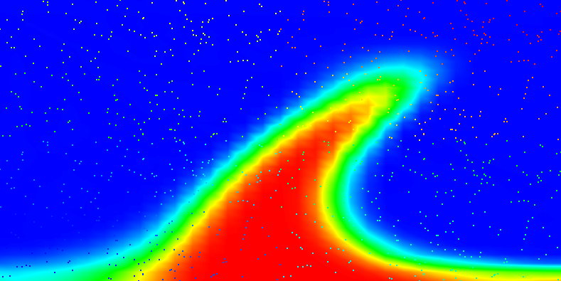
The particles shown here are not too impressive in still pictures since they are colorized by their particle number, which does not carry any particular meaning other than the fact that it enumerates the particles.27 The particle “id” can, however, be useful when viewing an animation of time steps. There, the different colors of particles allows the eye to follow the motion of a single particle. This is especially true if, after some time, particles have become well mixed by the flow field and adjacent particles no longer have similar colors. In any case, viewing such animations makes it rather intuitive to understand a flow field, but it can of course not be reproduced in a static medium such as this manual.
In any case, we will see in the next section how to attach more interesting information to particles, and how to visualize these.
Using particle properties. The particles in the above example only fulfil the purpose of visualizing the convection pattern. A more meaningful use for particles is to attach “properties” to them. A property consists of one or more numbers (or vectors or tensors) that may either be set at the beginning of the model run and stay constant, or are updated during the model runtime. These properties can then be used for many applications, e.g., storing an initial property (like the position, or initial composition), evaluating a property at a defined particle path (like the pressure-temperature evolution of a certain piece of rock), or by integrating a quantity along a particle path (like the integrated strain a certain domain has experienced). We illustrate these properties in the cookbook cookbooks/composition-_passive-_particles-_properties.prm, in which we add the following lines to the Particles subsection (we also increase the number of particles compared to the previous section to make the visualizations below more obvious):
These commands make sure that every particle will carry four different properties (function, pT path, initial position and initial composition), some of which may be scalars and others can have multiple components. (A full list of particle properties that can currently be selected can be found in Section ??, and new particle properties can be added as plugins as described in Section 6.2.) The properties selected above do the following:
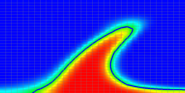
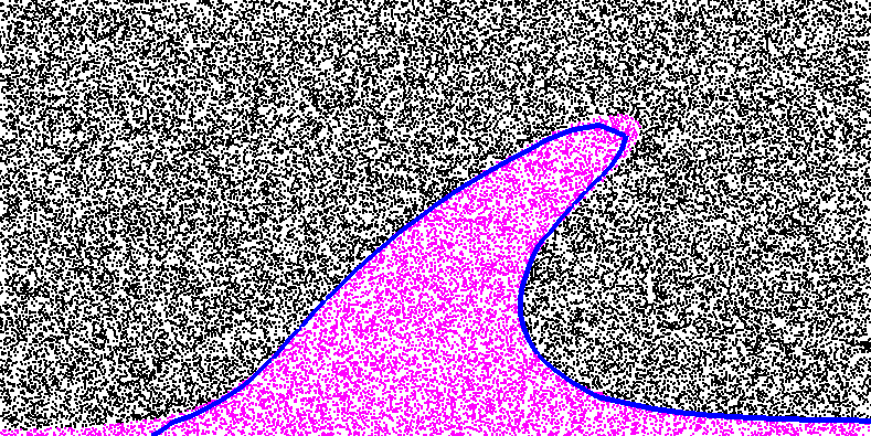
The results of all of these properties can of course be visualized. Fig. 24 shows some of the pictures one can create with particles. The top row shows both the composition field (along with the mesh on which it is defined) and the corresponding “initial ” particle property, at . Because the compositional field does not undergo any reactions, it should of course simply be the initial composition advected along with the flow field, and therefore equal the values of the corresponding particle property. However, field-based compositions suffer from diffusion. On the other hand, the amount of diffusion can easily be decreased by mesh refinement.
The bottom of the figure shows the norm of the “initial position” property at the initial time and at time . These images therefore show how far from the origin each of the particles shown was at the initial time.
Using active particles. In the examples above, particle properties passively track distinct model properties. These particle properties, however, may also be used to actively influence the model as it runs. For instance, a composition-dependent material model may use particles’ initial composition rather than an advected compositional field. To make this work – i.e., to get information from particles that are located at unpredictable locations, to the quadrature points at which material models and other parts of the code need to evaluate these properties – we need to somehow get the values from particles back to fields that can then be evaluated at any point where this is necessary. A slightly modified version of the active-composition cookbook (cookbooks/composition-_active.prm) illustrates how to use ‘active particles’ in this manner.
This cookbook, cookbooks/composition-_active-_particles.prm, modifies two sections of the input file. First, particles are added under the Postprocess section:
Here, each particle will carry the velocity and initial composition properties. In order to use the particle initial composition value to modify the flow through the material model, we now modify the Composition section:
What this does is the following: It says that there will be two compositional fields, called lower and upper (because we will use them to indicate material that comes from either the lower or upper part of the domain). Next, the Compositional field methods states that each of these fields will be computed by interpolation from the particles (if we had left this parameter at its default value, field, for each field, then it would have solved an advection PDE in each time step, as we have done in all previous examples).
In this case, we specify that both of the compositional fields are in fact interpolated from particle properties in each time step. How this is done is described in the fourth line. To understand it, it is important to realize that particles and fields have matching names: We have named the fields lower and upper, whereas the properties that result from the initial composition entry in the particles section are called initial lower and initial upper, since they inherit the names of the fields.
The syntax for interpolation from particles to fields then states that the lower field will be set to the interpolated value of the initial lower particle property at the end of each time step, and similarly for the upper field. In turn, the initial composition particle property was using the same method that one would have used for the compositional field initialization if these fields were actually advected along in each time step.
In this model the given global refinement level (5), associated number of cells (1024) and 100,000 total particles produces an average particle-per-cell count slightly below 100. While on the high end compared to most geodynamic studies using active particles, increasing the number of particles per cell further may alter the solution. As with the numerical resolution, any study using active particles should systematically vary the number of particles per cell in order to determine this parameter’s influence on the simulation.
This section was contributed by Ian Rose.
Free surfaces are numerically challenging but can be useful for self consistently tracking dynamic topography and may be quite important as a boundary condition for tectonic processes like subduction. The parameter file cookbooks/free-_surface.prm provides a simple example of how to set up a model with a free surface, as well as demonstrates some of the challenges associated with doing so.
ASPECT supports models with a free surface using an Arbitrary Lagrangian-Eulerian framework (see Section 2.12). Most of this is done internally, so you do not need to worry about the details to run this cookbook. Here we demonstrate the evolution of surface topography that results when a blob of hot material rises in the mantle, pushing up the free surface as it does. Usually the amplitude of free surface topography will be small enough that it is difficult to see with the naked eye in visualizations, but the topography postprocessor can help by outputting the maximum and minimum topography on the free surface at every time step.
The bulk of the parameter file for this cookbook is similar to previous ones in this manual. We use initial temperature conditions that set up a hot blob of rock in the center of the domain.
The main addition is the Free surface subsection. In this subsection you need to give ASPECT a comma separated list of the free surface boundary indicators. In this case, we are dealing with the ‘top’ boundary of a box in 2D. There is another significant parameter that needs to be set here: the value for the stabilization parameter “theta”. If this parameter is zero, then there is no stabilization, and you are likely to see instabilities develop in the free surface. If this parameter is one then it will do a good job of stabilizing the free surface, but it may overly damp its motions. The default value is 0.5.
Also worth mentioning is the change to the CFL number. Stability concerns typically mean that when making a model with a free surface you will want to take smaller time steps. In general just how much smaller will depend on the problem at hand as well as the desired accuracy.
Following are the sections in the input file specific to this testcase. The full parameter file may be found at cookbooks/free-_surface.prm.
Running this input file will produce results like those in Figure 25. The model starts with a single hot blob of rock which rises in the domain. As it rises, it pushes up the free surface in the middle, creating a topographic high there. This is similar to the kind of dynamic topography that you might see above a mantle plume on Earth. As the blob rises and diffuses, it loses the buoyancy to push up the boundary, and the surface begins to relax.
After running the cookbook, you may modify it in a number of ways:

This section was contributed by William Durkin.
This cookbook is a modification of the previous example that explores changes in the way topography develops when a highly viscous crust is added. In this cookbook, we use a material model in which the material changes from low viscosity mantle to high viscosity crust at , i.e., the piecewise viscosity function is defined as
where and are the viscosities of the upper and lower layers, respectively. This viscosity model can be implemented by creating a plugin that is a small modification of the simpler material model (from which it is otherwise simply copied). We call this material model “SimplerWithCrust”. In particular, what is necessary is an evaluation function that looks like this:
Additional changes make the new parameters Jump height, Lower viscosity, and Upper viscosity available to the input parameter file, and corresponding variables available in the class and used in the code snippet above. The entire code can be found in cookbooks/free-_surface-_with-_crust/plugin/simpler-_with-_crust.cc. Refer to Section 6.1 for more information about writing and running plugins.
The following changes are necessary compared to the input file from the cookbook shown in Section 5.2.6 to include a crust:
Note that the height of the interface at 170km is interpreted in the coordinate system in which the box geometry of this cookbook lives. The box has dimensions , so an interface height of 170km implies a depth of 30km.
The entire script is located in cookbooks/free-_surface-_with-_crust/free-_surface-_with-_crust.prm.
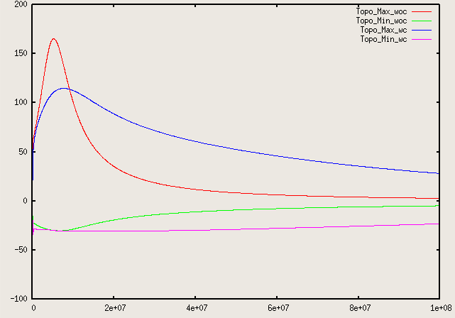
Running this input file yields a crust that is 30km thick and 1000 times as viscous as the lower layer. Figure 26 shows that adding a crust to the model causes the maximum topography to both decrease and occur at a later time. Heat flows through the system primarily by advection until the temperature anomaly reaches the base of the crustal layer (approximately at the time for which Fig 26 shows the temperature profile). The crust’s high viscosity reduces the temperature anomaly’s velocity substantially, causing it to affect the surface topography at a later time. Just as the cookbook shown in Section 5.2.6, the topography returns to zero after some time.

The original motivation for the functionality discussed here, as well as the setup of the input file, were provided by Cedric Thieulot.
Geophysical models are often characterized by abrupt and large jumps in material properties, in particular in the viscosity. An example is a subducting, cold slab surrounded by the hot mantle: Here, the strong temperature-dependence of the viscosity will lead to a sudden jump in the viscosity between mantle and slab. The length scale over which this jump happens will be a few or a few tens of kilometers. Such length scales cannot be adequately resolved in three-dimensional computations with typical meshes for global computations.
Having large viscosity variations in models poses a variety of problems to numerical computations. First, you will find that they lead to very long compute times because our solvers and preconditioners break down. This may be acceptable if it would at least lead to accurate solutions, but large viscosity gradients lead also to large pressure gradients, and this in turn leads to over- and undershoots in the numerical approximation of the gradient. We will demonstrate both of these issues experimentally below.
One of the solution to such problems is the realization that one can mitigate some of the effects by averaging material properties on each cell somehow (see, for example, [SBE08, DK08, DMGT11, Thi15, TMK14]). Before going into detail, it is important to realize that if we choose material properties not per quadrature point when doing the integrals for forming the finite element matrix, but per cell, then we will lose accuracy in the solution in those cases where the solution is smooth. More specifically, we will likely lose one or more orders of convergence. In other words, it would be a bad idea to do this averaging unconditionally. On the other hand, if the solution has essentially discontinuous gradients and kinks in the velocity field, then at least at these locations we cannot expect a particularly high convergence order anyway, and the averaging will not hurt very much either. In cases where features of the solution that are due to strongly varying viscosities or other parameters, dominate, we may then as well do the averaging per cell.
To support such cases, ASPECT supports an operation where we evaluate the material model at every quadrature point, given the temperature, pressure, strain rate, and compositions at this point, and then either (i) use these values, (ii) replace the values by their arithmetic average , (iii) replace the values by their harmonic average , (iv) replace the values by their geometric average , or (v) replace the values by the largest value over all quadrature points on this cell. Option (vi) is to project the values from the quadrature points to a bi- (in 2d) or trilinear (in 3d) finite element space on every cell, and then evaluate this finite element representation again at the quadrature points. Unlike the other five operations, the values we get at the quadrature points are not all the same here.
We do this operation for all quantities that the material model computes, i.e., in particular, the viscosity, the density, the compressibility, and the various thermal and thermodynamic properties. In the first 4 cases, the operation guarantees that the resulting material properties are bounded below and above by the minimum and maximum of the original data set. In the last case, the situation is a bit more complicated: The nodal values of the projection are not necessarily bounded by the minimal or maximal original values at the quadrature points, and then neither are the output values after re-interpolation to the quadrature points. Consequently, after projection, we limit the nodal values of the projection to the minimal and maximal original values, and only then interpolate back to the quadrature points.
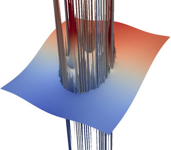
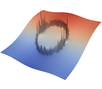
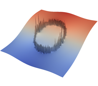
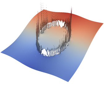
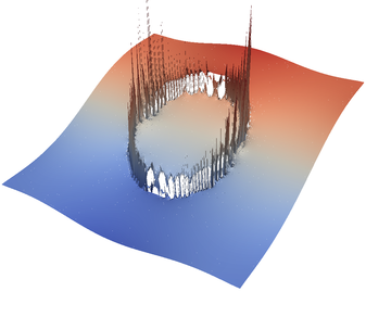
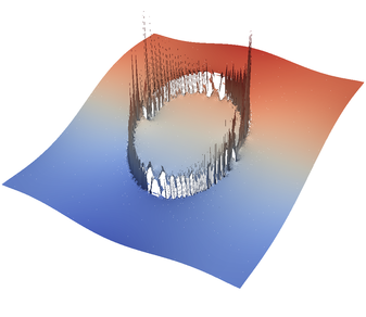
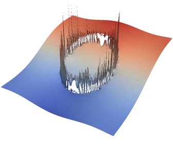
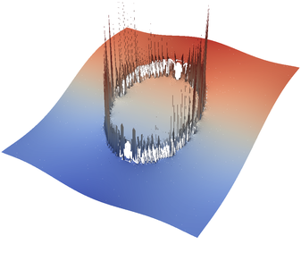
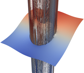
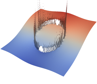
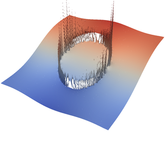
We demonstrate the effect of all of this with the “sinker” benchmark. This benchmark is defined by a high-viscosity, heavy sphere at the center of a two-dimensional box. This is achieved by defining a compositional field that is one inside and zero outside the sphere, and assigning a compositional dependence to the viscosity and density. We run only a single time step for this benchmark. This is all modeled in the following input file that can also be found in cookbooks/sinker-_with-_averaging/sinker-_with-_averaging.prm:
The type of averaging on each cell is chosen using this part of the input file:
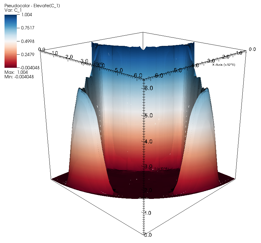
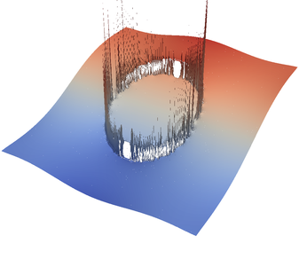
For the various different averaging options, and for different levels of mesh refinement, Fig. 27 shows pressure plots that illustrate the problem with oscillations of the discrete pressure. The important part of these plots is not that the solution looks discontinuous – in fact, the exact solution is discontinuous at the edge of the circle28 – but the spikes that go far above and below the “cliff” in the pressure along the edge of the circle. Without averaging, these spikes are obviously orders of magnitude larger than the actual jump height. The spikes do not disappear under mesh refinement nor averaging, but they become far less pronounced with averaging. The results shown in the figure do not really allow to draw conclusions as to which averaging approach is the best; a discussion of this question can also be found in [SBE08, DK08, DMGT11, TMK14]).
A very pleasant side effect of averaging is that not only does the solution become better, but it also becomes cheaper to compute. Table 2 shows the number of outer GMRES iterations when solving the Stokes equations (1)–(2).29 The implication of these results is that the averaging gives us a solution that not only reduces the degree of pressure over- and undershoots, but is also significantly faster to compute: for example, the total run time for 8 global refinement steps is reduced from 5,250s for no averaging to 358s for harmonic averaging.
 |  |  |  |  |  |
 |  |  |  |  |  |
| # of global | no averaging | arithmetic | harmonic | geometric | pick | project |
| refinement steps | averaging | averaging | averaging | largest | to | |
| 4 | 30+64 | 30+13 | 30+10 | 30+12 | 30+13 | 30+15 |
| 5 | 30+87 | 30+14 | 30+13 | 30+14 | 30+14 | 30+16 |
| 6 | 30+171 | 30+14 | 30+15 | 30+14 | 30+15 | 30+17 |
| 7 | 30+143 | 30+27 | 30+28 | 30+26 | 30+26 | 30+28 |
| 8 | 30+188 | 30+27 | 30+26 | 30+27 | 30+28 | 30+28 |
Such improvements carry over to more complex and realistic models. For example, in a simulation of flow under the East African Rift by Sarah Stamps, using approximately 17 million unknowns and run on 64 processors, the number of outer and inner iterations is reduced from 169 and 114,482 without averaging to 77 and 23,180 with harmonic averaging, respectively. This translates into a reduction of run-time from 145 hours to 17 hours. Assessing the accuracy of the answers is of course more complicated in such cases because we do not know the exact solution. However, the results without and with averaging do not differ in any significant way.
A final comment is in order. First, one may think that the results should be better in cases of discontinuous pressures if the numerical approximation actually allowed for discontinuous pressures. This is in fact possible: We can use a finite element in which the pressure space contains piecewise constants (see Section ??). To do so, one simply needs to add the following piece to the input file:
Disappointingly, however, this makes no real difference: the pressure oscillations are no better (maybe even worse) than for the standard Stokes element we use, as shown in Fig. 28 and Table 3. Furthermore, as shown in Table 4, the iteration numbers are also largely unaffected if any kind of averaging is used – though they are far worse using the locally conservative discretization if no averaging has been selected. On the positive side, the visualization of the discontinuous pressure finite element solution makes it much easier to see that the true pressure is in fact discontinuous along the edge of the circle.
| # of global | no averaging | arithmetic | harmonic | geometric | pick | project |
| refinement steps | averaging | averaging | averaging | largest | to | |
| 4 | 66.32 | 2.66 | 2.893 | 1.869 | 3.412 | 3.073 |
| 5 | 81.06 | 3.537 | 4.131 | 3.997 | 3.885 | 3.991 |
| 6 | 75.98 | 4.596 | 4.184 | 4.618 | 4.568 | 5.093 |
| 7 | 84.36 | 4.677 | 5.286 | 4.362 | 4.635 | 5.145 |
| 8 | 83.96 | 5.701 | 5.664 | 4.686 | 5.524 | 6.42 |
| # of global | no averaging | arithmetic | harmonic | geometric | pick | project |
| refinement steps | averaging | averaging | averaging | largest | to | |
| 4 | 30+376 | 30+16 | 30+12 | 30+14 | 30+14 | 30+17 |
| 5 | 30+484 | 30+16 | 30+14 | 30+14 | 30+14 | 30+16 |
| 6 | 30+583 | 30+16 | 30+17 | 30+14 | 30+17 | 30+17 |
| 7 | 30+1319 | 30+27 | 30+28 | 30+26 | 30+28 | 30+28 |
| 8 | 30+1507 | 30+28 | 30+27 | 30+28 | 30+28 | 30+29 |
This section was contributed by Jonathan Perry-Houts
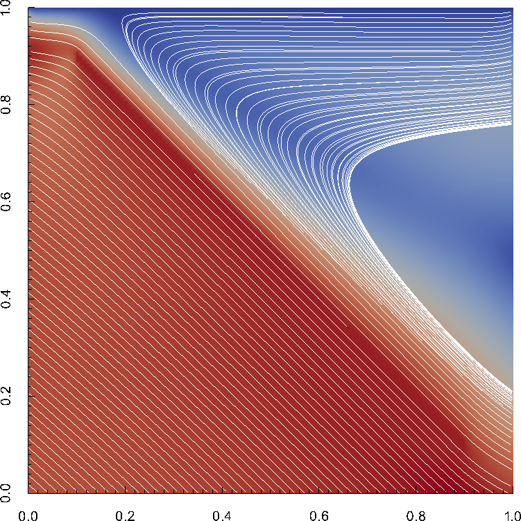
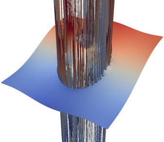
In cases where it is desirable to investigate the behavior of one part of the model domain but the controlling physics of another part is difficult to capture, such as corner flow in subduction zones, it may be useful to force the desired behavior in some parts of the model domain and solve for the resulting flow everywhere else. This is possible through the use of ASPECT’s “signal” mechanism, as documented in Section 6.5.
Internally, ASPECT adds “constraints” to the finite element system for boundary conditions and hanging nodes. These are places in the finite element system where certain solution variables are required to match some prescribed value. Although it is somewhat mathematically inadmissible to prescribe constraints on nodes inside the model domain, , it is nevertheless possible so long as the prescribed velocity field fits in to the finite element’s solution space, and satisfies the other constraints (i.e., is divergence free).
Using ASPECT’s signals mechanism, we write a shared library which provides a “slot” that listens for the signal which is triggered after the regular model constraints are set, but before they are “distributed.”
As an example of this functionality, below is a plugin which allows the user to prescribe internal velocities with functions in a parameter file:
The above plugin can be compiled with cmake . && make in the cookbooks/prescribed_velocity directory. It can be loaded in a parameter file as an “Additional shared library.” By setting parameters like those shown below, it is possible to produce many interesting flow fields such as the ones visualized in (Figure 29).
(a) |
(b) |
This section was contributed by Ryan Grove
Standard finite element discretizations of advection-diffusion equations introduce unphysical oscillations around steep gradients. Therefore, stabilization must be added to the discrete formulation to obtain correct solutions. In ASPECT, we use the Entropy Viscosity scheme developed by Guermond et al. in the paper [Jea11]. In this scheme, an artificial viscosity is calculated on every cell and used to try to combat these oscillations that cause unwanted overshoot and undershoot. More information about how ASPECT does this is located at https://dealii.org/developer/doxygen/deal.II/step_31.html.
Instead of just looking at an individual cell’s artificial viscosity, improvements in the minimizing of the oscillations can be made by smoothing. Smoothing is the act of finding the maximum artificial viscosity taken over a cell and the neighboring cells across the faces of , i.e.,
where is the set containing and the neighbors across the faces of .
This feature can be turned on by setting the ?? flag inside the ?? subsection inside the ?? subsection in your parameter file.
To show how this can be used in practice, let us consider the simple convection in a quarter of a 2d annulus cookbook in Section 5.3.1, a radial compositional field was added to help show the advantages of using the artificial viscosity smoothing feature.
By applying the following changes shown below to the parameters of the already existing file
it is possible to produce pictures of the simple convection in a quarter of a 2d annulus such as the ones visualized in Figure 30.

(a) |
(b) |
This section was contributed by Juliane Dannberg and Rene Gassmöller
In many geophysical settings, material properties, and in particular the rheology, do not only depend on the current temperature, pressure and strain rate, but also on the history of the system. This can be incorporated in ASPECT models by tracking history variables through compositional fields. In this cookbook, we will show how to do this by tracking the strain that idealized little grains of finite size accumulate over time at every (Lagrangian) point in the model.
Here, we use a material model plugin that defines the compositional fields as the components of the deformation gradient tensor , and modifies the right-hand side of the corresponding advection equations to accumulate strain over time. This is done by adjusting the out.reaction_terms variable:
Let us denote the accumulated deformation at time step as . We can calculate its time derivative as the product of two tensors, namely the current velocity gradient and the deformation gradient accumulated up to the previous time step, in other words , and , with being the identity tensor. While we refer to other studies [MJ83, DT98, BKEO03] for a derivation of this relationship, we can give an intuitive example for the necessity to apply the velocity gradient to the already accumulated deformation, instead of simply integrating the velocity gradient over time. Consider a simple one-dimensional “grain” of length , in which case the deformation tensor only has one component, the compression in -direction. If one embeds this grain into a convergent flow field for a compressible medium where the dimensionless velocity gradient is (e.g. a velocity of zero at its left end at , and a velocity of at its right end at ), simply integrating the velocity gradient would suggest that the grain reaches a length of zero after two units of time, and would then “flip” its orientation, which is clearly non-physical. What happens instead can be seen by solving the equation of motion for the right end of the grain . Solving this equation for leads to . This is therefore also the solution for since transforms the initial position of into the deformed position of , which is the definition of .
In more general cases a visualization of is not intuitive, because it contains rotational components that represent a rigid body rotation without deformation. Following [BKEO03] we can polar-decompose the tensor into a positive-definite and symmetric left stretching tensor , and an orthogonal rotation tensor , as , therefore . The left stretching tensor (or finite strain tensor) then describes the deformation we are interested in, and its eigenvalues and eigenvectors describe the length and orientation of the half-axes of the finite strain ellipsoid. Moreover, we will represent the amount of relative stretching at every point by the ratio , called the natural strain [Rib92].
The full plugin implementing the integration of can be found in cookbooks/finite_strain/finite_strain.cc and can be compiled with cmake . && make in the cookbooks/finite_strain directory. It can be loaded in a parameter file as an “Additional shared library”, and selected as material model. As it is derived from the “simple” material model, all input parameters for the material properties are read in from the subsection Simple model.
The plugin was tested against analytical solutions for the deformation gradient tensor in simple and pure shear as described in benchmarks/finite_strain/pure_shear.prm and benchmarks/finite_strain/simple_shear.prm.
We will demonstrate its use at the example of a 2D Cartesian convection model (Figure 31): Heating from the bottom leads to the ascent of plumes from the boundary layer (top panel), and the amount of stretching is visible in the distribution of natural strain (color in lower panel). Additionally, the black crosses show the direction of stretching and compression (the eigenvectors of ). Material moves to the sides at the top of the plume head, so that it is shortened in vertical direction (short vertical lines) and stretched in horizontal direction (long horizontal lines). The sides of the plume head show the opposite effect. Shear occurs mostly at the edges of the plume head, in the plume tail, and in the bottom boundary layer (black areas in the natural strain distribution).
The example used here shows how history variables can be integrated up over the model evolution. While we do not use these variables actively in the computation (in our example, there is no influence of the accumulated strain on the rheology or any other material property), it would be trivial to extend this material model in a way that material properties depend on the integrated strain: Because the values of the compositional fields are part of what the material model gets as inputs, they can easily be used for computing material model outputs such as the viscosity.
This section was contributed by Juliane Dannberg
Many geophysical setups require initial conditions with several different materials and complex geometries. Hence, sometimes it would be easier to generate the initial geometries of the materials as a drawing instead of by writing code. The MATLAB-based library geomIO (http://geomio.bitbucket.org/) provides a convenient tool to convert a drawing generated with the vector graphics editor Inkscape (https://inkscape.org/en/) to a data file that can be read into ASPECT. Here, we will demonstrate how this can be done for a 2D setup for a model with one compositional field, but geomIO also has the capability to create 3D volumes based on a series of 2D vector drawings using any number of different materials. Similarly, initial conditions defined in this way can also be used with particles instead of compositional fields.
To obtain the developer version of geomIO, you can clone the bitbucket repository by executing the command
or you can download geomIO here. You will then need to add the geomIO source folders to your MATLAB path by running the file located in /path/to/geomio/installation/InstallGeomIO.m. An extensive documentation for how to use geomIO can be found here. Among other things, it explains how to generate drawings in Inkscape that can be read in by geomIO, which involves assigning new attributes to paths in Inkscape’s XML editor. In particular, a new property ‘phase’ has to be added to each path, and set to a value corresponding to the index of the material that should be present in this region in the initial condition of the geodynamic model.
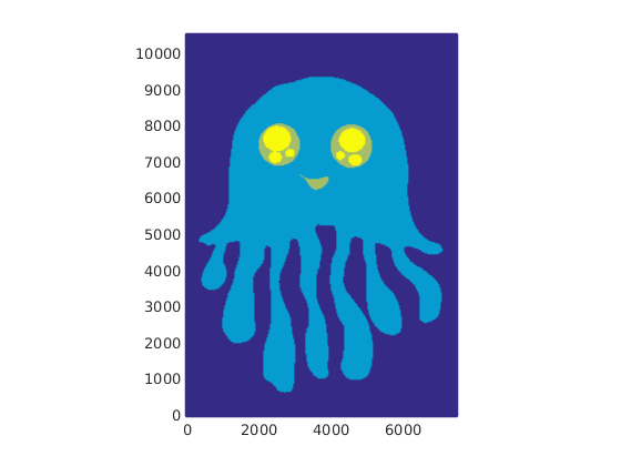
We will here use a drawing of a jellyfish located in cookbooks/geomio/jellyfish.svg, where different phases have already been assigned to each path (Figure 32).
After geomIO is initialized in MATLAB, we run geomIO as described in the documentation, loading the default options and then specifying all the option we want to change, such as the path to the input file, or the resolution:
You can view all of the options available by typing opt in MATLAB.
In the next step we create the grid that is used for the coordinates in the ascii data initial conditions file and assign a phase to each grid point:
You can plot the Phase variable in MATLAB to see if the drawing was read in and all phases are assigned correctly (Figure 33).
Finally, we want to write output in a format that can be read in by ASPECT’s ascii data compositional initial conditions plugin. We write the data into the file jelly.txt:
To read in the file we just created (a copy is located in ASPECT’s data directory), we set up a model with a box geometry with the same extents we specified for the drawing in px and one compositional field. We choose the ascii data compositional initial conditions and specify that we want to read in our jellyfish. The relevant parts of the input file are listed below:
If we look at the output in paraview, we can see our jellyfish, with the mesh refined at the boundaries between the different phases (Figure 34).
For a geophysical setup, the MATLAB code could be extended to write out the phases into several different columns of the ASCII data file (corresponding to different compositional fields). This initial conditions file could then be used in ASPECT with a material model such as the multicomponent model, assigning each phase different material properties.
An animation of a model using the jellyfish as initial condition and assigning it a higher viscosity can be found here: https://www.youtube.com/watch?v=YzNTubNG83Q.
19This difference is far smaller than the numerical error in the heat flux on the mesh this data is computed on.
20The statistics file gives this value to more digits: 4.89008498. However, these are clearly more digits than the result is accurate.
21For computations of this size, one should test a few time steps in debug mode but then, of course, switch to running the actual computation in optimized mode – see Section 4.3.
22Note that the statistics file actually contains the outward heat flux for each of the six boundaries, which corresponds to the negative of upward flux for the bottom boundary. The figure therefore shows the negative of the values available in the statistics file.
23In fact, the pictures are generated using a twice more refined mesh to provide adequate resolution. We keep the default setting of five global refinements in the parameter file as documented above to keep compute time reasonable when using the default settings.
24Of course, this interpretation suggests that we could have achieved the same goal by encoding everything into a single function – that would, for example, have had initial values one, zero and minus one in the three parts of the domain we are interested in.
25We note that this is no different for particles where the position of particles has to be integrated over time and is subject to numerical error. In simulations, their location is therefore not the exact one but also subject to a diffusive process resulting from numerical inaccuracies. Furthermore, in long thin filaments, the number of particles per cell often becomes too small and new particles have to be inserted; their properties are then interpolated from the surrounding particles, a process that also incurs a smoothing penalty.
26The actual values do not matter as much here. They are chosen in such a way that the system – previously driven primarily by the velocity boundary conditions at the top – now also feels the impact of the density variations. To have an effect, the buoyancy induced by the density difference between materials must be strong enough to balance or at least approach the forces exerted by whatever is driving the velocity at the top.
27Particles are enumerated in a way so that first the first processor in a parallel computations numbers all of the particles on its first cell, then its second cell, and so on; then the second processor does the same with particles in the order of the cells it owns; etc. Thus, the “id” shown in the picture is not just a random number, but rather shows the order of cells and how they belonged to the processors that participated in the computation at the time when particles were created. After some time, particles may of course have become well mixed. In any case, this ordering is of no real practical use.
28This is also easy to try experimentally – use the input file from above and select 5 global and 10 adaptive refinement steps, with the refinement criteria set to density, then visualize the solution.
29The outer iterations are only part of the problem. As discussed in [KHB12], each GMRES iteration requires solving a linear system with the elliptic operator . For highly heterogeneous models, such as the one discussed in the current section, this may require a lot of Conjugate Gradient iterations. For example, for 8 global refinement steps, the 30+188 outer iterations without averaging shown in Table 2 require a total of 22,096 inner CG iterations for the elliptic block (and a total of 837 for the approximate Schur complement). Using harmonic averaging, the 30+26 outer iterations require only 1258 iterations on the elliptic block (and 84 on the Schur complement). In other words, the number of inner iterations per outer iteration (taking into account the split into “cheap” and “expensive” outer iterations, see [KHB12]) is reduced from 117 to 47 for the elliptic block and from 3.8 to 1.5 for the Schur complement.


