5.3 Geophysical setups
Having gone through the ways in which one can set up problems in rectangular geometries, let us now move on to
situations that are directed more towards the kinds of things we want to use ASPECT for: the simulation of
convection in the rocky mantles of planets or other celestial bodies.
To this end, we need to go through the list of issues that have to be described and that were outlined in
Section 5.1, and address them one by one:
- What internal forces act on the medium (the equation)? This may in fact be the most difficult to answer
part of it all. The real material in Earth’s mantle is certainly no Newtonian fluid where the stress is a
linear function of the strain with a proportionality constant (the viscosity)
that only depends on the temperature. Rather, the real viscosity almost surely also depends on the
pressure and the strain rate. Because the issue is complicated and the exact material model not entirely
clear, for the next few subsections we will therefore ignore the issue and start with just using the
“simple” material model where the viscosity is constant and most other coefficients depend at most on
the temperature.
- What external forces do we have (the right hand side) There are of course other issues: for example,
should the model include terms that describe shear heating? Should it be compressible? Adiabatic
heating due to compression? Most of the terms that pertain to these questions appear on the right hand
sides of the equations, though some (such as the compressibility) also affect the differential operators
on the left. Either way, for the moment, let us just go with the simplest models and come back to the
more advanced questions in later examples.
One right hand side that will certainly be there is that due to gravitational acceleration. To first order,
within the mantle gravity points radially inward and has a roughly constant magnitude. In reality, of
course, the strength and direction of gravity depends on the distribution and density of materials in
Earth – and, consequently, on the solution of the model at every time step. We will discuss some of
the associated issues in the examples below.
- What is the domain (geometry)? This question is easier to answer. To first order, the domains we want
to simulate are spherical shells, and to second order ellipsoid shells that can be obtained by considering
the isopotential surface of the gravity field of a homogeneous, rotating fluid. A more accurate description
is of course the geoid for which several parameterizations are available. A complication arises if we ask
whether we want to include the mostly rigid crust in the domain and simply assume that it is part of
the convecting mantle, albeit a rather viscous part due to its low temperature and the low pressure
there, or whether we want to truncate the computation at the asthenosphere.
- What happens at the boundary for each variable involved (boundary conditions)? The mantle has two
boundaries: at the bottom where it contacts the outer core and at the top where it either touches
the air or, depending on the outcome of the discussion of the previous question, where it contacts
the lithospheric crust. At the bottom, a very good approximation of what is happening is certainly
to assume that the velocity field is tangential (i.e., horizontal) and without friction forces due to the
very low viscosity of the liquid metal in the outer core. Similarly, we can assume that the outer core is
well mixed and at a constant temperature. At the top boundary, the situation is slightly more complex
because in reality the boundary is not fixed but also allows vertical movement. If we ignore this, we can
assume free tangential flow at the surface or, if we want, prescribe the tangential velocity as inferred
from plate motion models. ASPECT has a plugin that allows to query this kind of information from
the GPlates program.
- How did it look at the beginning (initial conditions)? This is of course a trick question. Convection in
the mantle of earth-like planets did not start with a concrete initial temperature distribution when the
mantle was already fully formed. Rather, convection already happened when primordial material was
still separating into mantle and core. As a consequence, for models that only simulate convection using
mantle-like geometries and materials, no physically reasonable initial conditions are possible that date
back to the beginning of Earth. On the other hand, recall that we only need initial conditions for the
temperature (and, if necessary, compositional fields). Thus, if we have a temperature profile at a given
time, for example one inferred from seismic data at the current time, then we can use these as the
starting point of a simulation.
This discussion shows that there are in fact many pieces with which one can play and for which the answers are
in fact not always clear. We will address some of them in the cookbooks below. Recall in the descriptions we use in
the input files that ASPECT uses physical units, rather than non-dimensionalizing everything. The advantage, of
course, is that we can immediately compare outputs with actual measurements. The disadvantage is that we need to
work a bit when asked for, say, the Rayleigh number of a simulation.
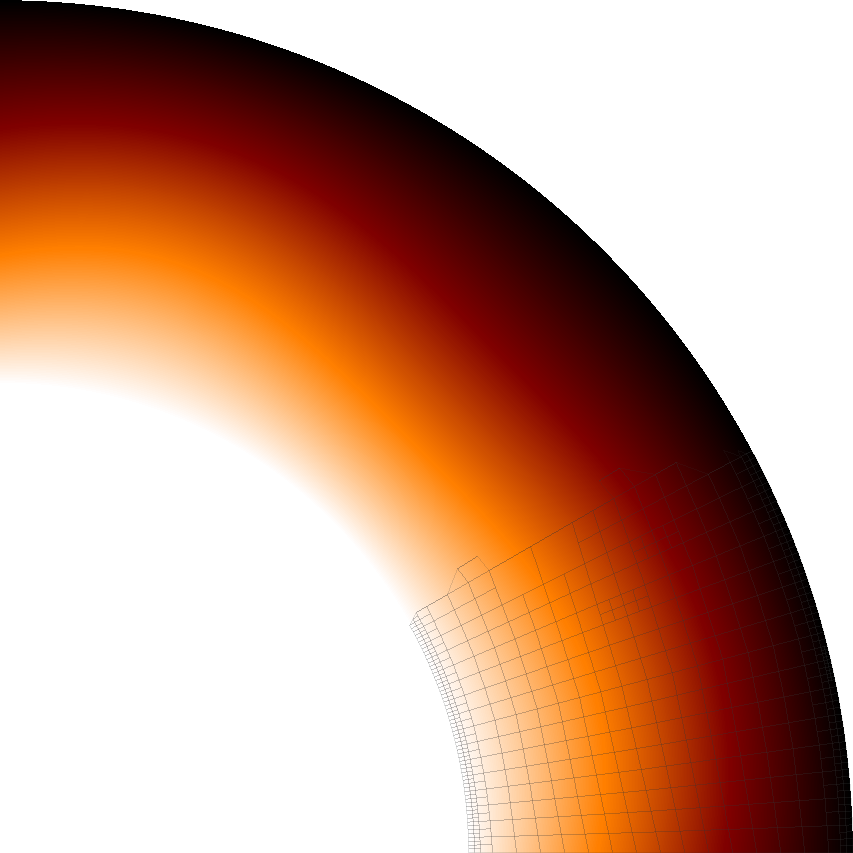
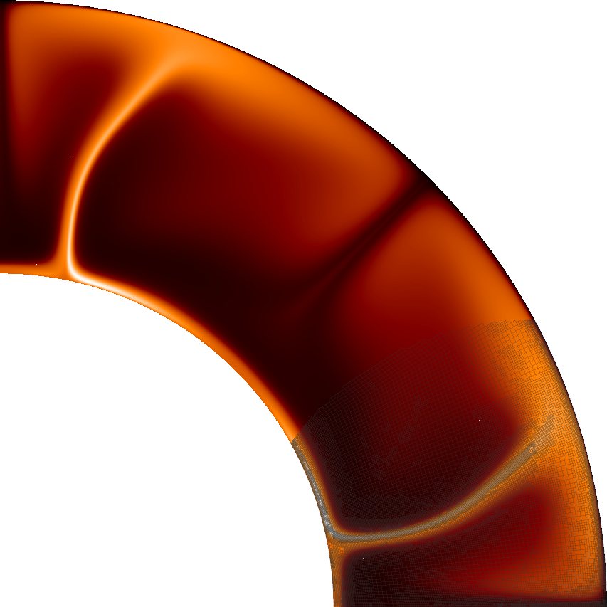
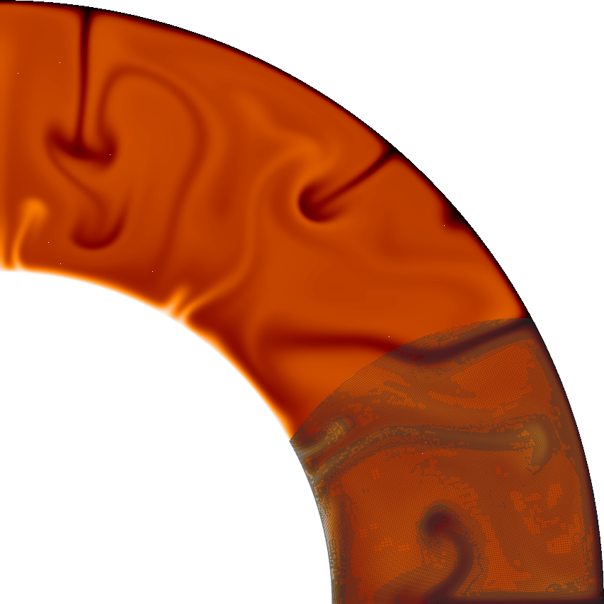
5.3.1 Simple convection in a quarter of a 2d annulus
Let us start this sequence of cookbooks using a simpler situation: convection in a quarter of a 2d
shell. We choose this setup because 2d domains allow for much faster computations (in turn allowing
for more experimentation) and because using a quarter of a shell avoids a pitfall with boundary
conditions we will discuss in the next section. Because it’s simpler to explain what we want to describe
in pictures than in words, Fig. 35 shows the domain and the temperature field at a few time
steps. In addition, you can find a movie of how the temperature evolves over this time period at
http://www.youtube.com/watch?v=d4AS1FmdarU.
Let us just start by showing the input file (which you can find in cookbooks/shell_simple_2d.prm):
In the following, let us pick apart this input file:
- Lines 1–4 are just global parameters. Since we are interested in geophysically realistic simulations, we
will use material parameters that lead to flows so slow that we need to measure time in years, and we
will set the end time to 1.5 billion years – enough to see a significant amount of motion.
- The next block (lines 7–14) describes the material that is convecting (for historical reasons, the
remainder of the parameters that describe the equations is in a different section, see the fourth point
below). We choose the simplest material model ASPECT has to offer where the viscosity is constant
(here, we set it to )
and so are all other parameters except for the density which we choose to be
with ,
and .
The remaining material parameters remain at their default values and you can find their values
described in the documentation of the simple material model in Sections ?? and ??.
- Lines 17–25 then describe the geometry. In this simple case, we will take a quarter of a 2d shell (recall
that the dimension had previously been set as a global parameter) with inner and outer radii matching
those of a spherical approximation of Earth.
- The second part of the model description and boundary values follows in lines 28–42. The boundary
conditions require us to look up how the geometry model we chose (the spherical shell model)
assigns boundary indicators to the four sides of the domain. This is described in Section ?? where
the model announces that boundary indicator zero is the inner boundary of the domain, boundary
indicator one is the outer boundary, and the left and right boundaries for a 2d model with opening
angle of 90 degrees as chosen here get boundary indicators 2 and 3, respectively. In other words, the
settings in the input file correspond to a zero velocity at the inner boundary and tangential flow at all
other boundaries. We know that this is not realistic at the bottom, but for now there are of course many
other parts of the model that are not realistic either and that we will have to address in subsequent
cookbooks. Furthermore, the temperature is fixed at the inner and outer boundaries (with the left
and right boundaries then chosen so that no heat flows across them, emulating symmetry boundary
conditions) and, further down, set to values of 700 and 4000 degrees Celsius – roughly realistic for the
bottom of the crust and the core-mantle boundary.
- Lines 45–47 describe that we want a model where equation (3) contains the shear heating term
(noting that the default is to use an incompressible model for which the term
in the shear heating contribution is zero). Considering a reasonable choice of heating terms is not the
focus of this simple cookbook, therefore we will leave a discussion of possible and reasonable heating
terms to another cookbook.
- The description of what we want to model is complete by specifying that the initial temperature
is a perturbation with hexagonal symmetry from a linear interpolation between inner and outer
temperatures (see Section ??), and what kind of gravity model we want to choose (one reminiscent of
the one inside the Earth mantle, see Section ??).
- The remainder of the input file consists of a description of how to choose the initial mesh and how to
adapt it (lines 60–65) and what to do at the end of each time step with the solution that ASPECT
computes for us (lines 68–81). Here, we ask for a variety of statistical quantities and for graphical
output in VTU format every million years.
Note: Having described everything to ASPECT, you may want to view the video linked to above
again and compare what you see with what you expect. In fact, this is what one should always do
having just run a model: compare it with expectations to make sure that we have not overlooked
anything when setting up the model or that the code has produced something that doesn’t match
what we thought we should get. Any such mismatch between expectation and observed result
is typically a learning opportunity: it either points to a bug in our input file, or it provides us
with insight about an aspect of reality that we had not foreseen. Either way, accepting results
uncritically is, more often than not, a way to scientifically invalid results.
The model we have chosen has a number of inadequacies that make it not very realistic (some of those happened
more as an accident while playing with the input file and weren’t a purposeful experiment, but we left
them in because they make for good examples to discuss below). Let us discuss these issues in the
following.
Dimension.
This is a cheap shot but it is nevertheless true that the world is three-dimensional whereas the simulation here is
2d. We will address this in the next section.
Incompressibility, adiabaticity and the initial conditions.
This one requires a bit more discussion. In the model selected above, we have chosen a model that is
incompressible in the sense that the density does not depend on the pressure and only very slightly depends on the
temperature. In such models, material that rises up does not cool down due to expansion resulting from the pressure
dropping, and material that is transported down does not adiabatically heat up. Consequently, the adiabatic
temperature profile would be constant with depth, and a well-mixed model with hot inner and cold outer
boundary would have a constant temperature with thin boundary layers at the bottom and top of the
mantle. In contrast to this, our initial temperature field was a perturbation of a linear temperature
profile.
There are multiple implications of this. First, the temperature difference between outer and inner boundary of
3300 K we have chosen in the input file is much too large. The temperature difference that drives the convection, is
the difference in addition to the temperature increase a volume of material would experience if it were to be
transported adiabatically from the surface to the core-mantle boundary. This difference is much smaller than 3300 K
in reality, and we can expect convection to be significantly less vigorous than in the simulation here. Indeed, using
the values in the input file shown above, we can compute the Rayleigh number for the current case to
be
|
|
Second, the initial temperature profile we chose is not realistic – in fact, it is a completely unstable one: there is
hot material underlying cold one, and this is not just the result of boundary layers. Consequently, what happens in
the simulation is that we first overturn the entire temperature field with the hot material in the lower half of the
domain swapping places with the colder material in the top, to achieve a stable layering except for the boundary
layers. After this, hot blobs rise from the bottom boundary layer into the cold layer at the bottom of the mantle,
and cold blobs sink from the top, but their motion is impeded about half-way through the mantle once they reach
material that has roughly the same temperature as the plume material. This impedes convection until we reach a
state where these plumes have sufficiently mixed the mantle to achieve a roughly constant temperature
profile.
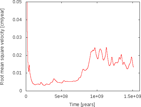
This effect is visible in the movie linked to above where convection does not penetrate the entire depth of the
mantle for the first 20 seconds (corresponding to roughly the first 800 million years). We can also see
this effect by plotting the root mean square velocity, see the left panel of Fig. 36. There, we can see
how the average velocity picks up once the stable layering of material that resulted from the initial
overturning has been mixed sufficiently to allow plumes to rise or sink through the entire depth of the
mantle.
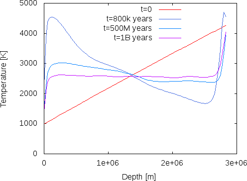
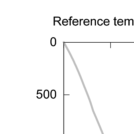
The right panel of Fig. 36 shows a different way of visualizing this, using the average temperature at various
depths of the model (this is what the depth average postprocessor computes). The figure shows how the initially
linear unstable layering almost immediately reverts completely, and then slowly equilibrates towards a temperature
profile that is constant throughout the mantle (which in the incompressible model chosen here equates to an
adiabatic layering) except for the boundary layers at the inner and outer boundaries. (The end points of these
temperature profiles do not exactly match the boundary values specified in the input file because we average
temperatures over shells of finite width.)
A conclusion of this discussion is that if we want to evaluate the statistical properties of the flow field, e.g., the
number of plumes, average velocities or maximal velocities, then we need to restrict our efforts to times after
approximately 800 million years in this simulation to avoid the effects of our inappropriately chosen initial
conditions. Likewise, we may actually want to choose initial conditions more like what we see in the model for later
times, i.e., constant in depth with the exception of thin boundary layers, if we want to stick to incompressible
models.
Material model.
The model we use here involves viscosity, density, and thermal property functions that do not depend on the
pressure, and only the density varies (slightly) with the temperature. We know that this is not the case in
nature.
Shear heating.
When we set up the input file, we started with a model that includes the shear heating term
in
eq. (3). In hindsight, this may have been the wrong decision, but it provides an opportunity to investigate whether
we think that the results of our computations can possibly be correct.
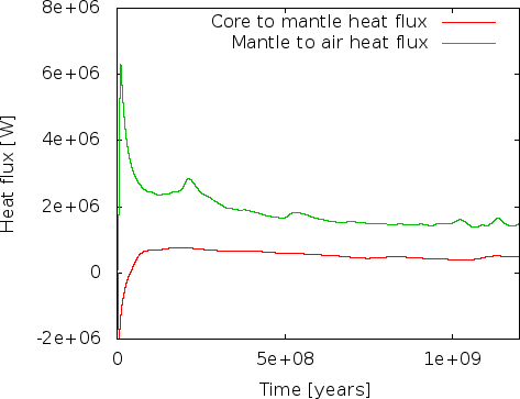
We first realized the issue when looking at the heat flux that the heat flux statistics postprocessor computes. This is shown in
the left panel of Fig. 37.
There are two issues one should notice here. The more obvious one is that the flux from the mantle to the air is
consistently higher than the heat flux from core to mantle. Since we have no radiogenic heating model selected (see
the List of model names parameter in the Heating model section of the input file; see also Section ??), in the
long run the heat output of the mantle must equal the input, unless is cools. Our misconception was that after the
800 million year transition, we believed that we had reached a steady state where the average temperature
remains constant and convection simply moves heat from the core-mantle boundary the surface. One
could also be tempted to believe this from the right panel in Fig. 36 where it looks like the average
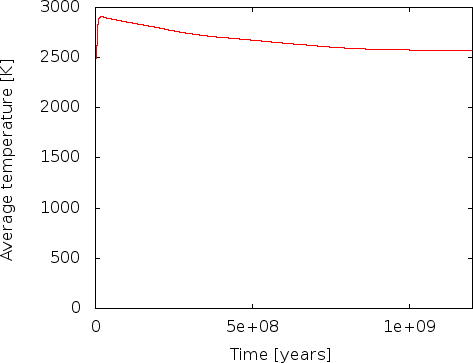
temperature does at least not change dramatically. But, it is easy to convince oneself that that is not the
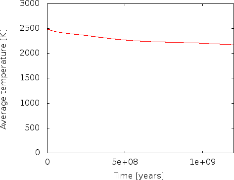
case: the temperature statistics postprocessor we had previously selected also outputs data about
the mean temperature in the model, and it looks like shown in the left panel of Fig. 38. Indeed, the
average temperature drops over the course of the 1.2 billion years shown here. We could now convince
ourselves that indeed the loss of thermal energy in the mantle due to the drop in average temperature is
exactly what fuels the persistently imbalanced energy outflow. In essence, what this would show is
that if we kept the temperature at the boundaries constant, we would have chosen a mantle that was
initially too hot on average to be sustained by the boundary values and that will cool until it will be in
energetic balance and on longer time scales, in- and outflow of thermal energy would balance each
other.
However, there is a bigger problem. Fig. 37 shows that at the very beginning, there is a spike in energy flux
through the outer boundary. We can explain this away with the imbalanced initial temperature field that leads to an
overturning and, thus, a lot of hot material rising close to the surface that will then lead to a high energy flux
towards the cold upper boundary. But, worse, there is initially a negative heat flux into the mantle from the core –
in other words, the mantle is losing energy to the core. How is this possible? After all, the hottest part of the mantle
in our initial temperature field is at the core-mantle boundary, no thermal energy should be flowing
from the colder overlying material towards the hotter material at the boundary! A glimpse of the
solution can be found in looking at the average temperature in Fig. 38: At the beginning, the average
temperature rises, and apparently there are parts of the mantle that become hotter than the 4273 K we have
given the core, leading to a downward heat flux. This heating can of course only come from the shear
heating term we have accidentally left in the model: at the beginning, the unstable layering leads to
very large velocities, and large velocities lead to large velocity gradients that in turn lead to a lot of
shear heating! Once the initial overturning has subsided, after say 100 million years (see the mean
velocity in Fig. 36), the shear heating becomes largely irrelevant and the cooling of the mantle indeed
begins.
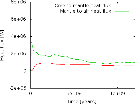
Whether this is really the case is of course easily verified: The right panels of Fig.s 37 and 38 show
heat fluxes and average temperatures for a model where we have switched off the shear heating by
setting
Indeed, doing so leads to a model where the heat flux from core to mantle is always positive, and where the
average temperature strictly drops!
Summary.
As mentioned, we will address some of the issues we have identified as unrealistic in the following sections.
However, despite all of this, some things are at least at the right order of magnitude, confirming that what
ASPECT is computing is reasonable. For example, the maximal velocities encountered in our model (after the 800
million year boundary) are in the range of 6–7cm per year, with occasional excursions up to 11cm. Clearly,
something is going in the right direction.
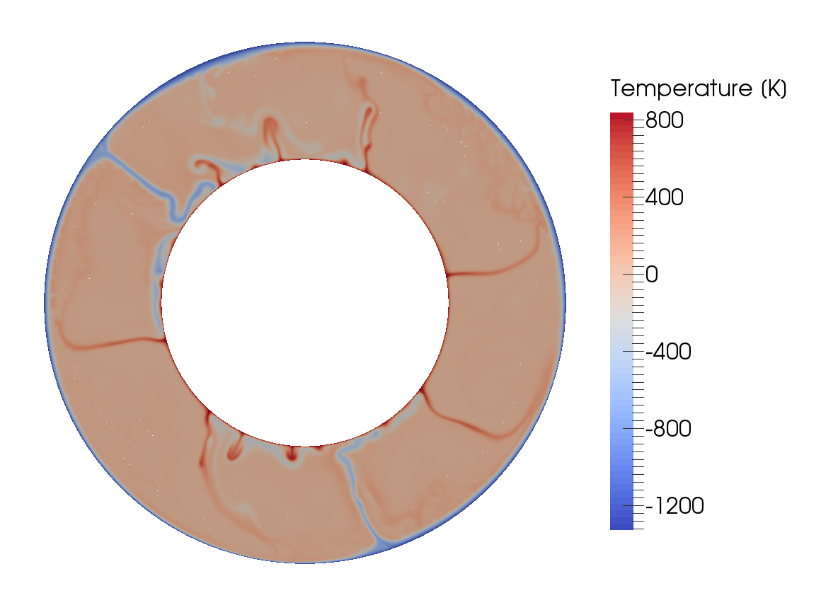
5.3.2 Simple convection in a spherical 3d shell
The setup from the previous section can of course be extended to 3d shell geometries as well – though at significant
computational cost. In fact, the number of modifications necessary is relatively small, as we will discuss below. To
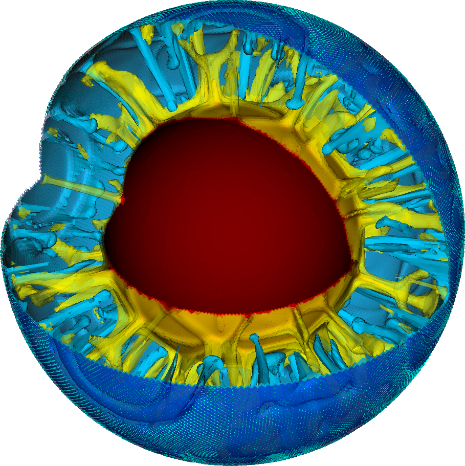
show an example up front, a picture of the temperature field one gets from such a simulation is shown in Fig. 39.
The corresponding movie can be found at http://youtu.be/j63MkEc0RRw.
The input file.
Compared to the input file discussed in the previous section, the number of changes is relatively small. However,
when taking into account the various discussions about which parts of the model were or were not realistic, they go
throughout the input file, so we reproduce it here in its entirety, interspersed with comments (the full input file can
also be found in cookbooks/shell_simple_3d.prm). Let us start from the top where everything looks the same
except that we set the dimension to 3:
The next section concerns the geometry. The geometry model remains unchanged at “spherical
shell” but we omit the opening angle of 90 degrees as we would like to get a complete spherical shell.
Such a shell of course also only has two boundaries (the inner one has indicator zero, the outer one
indicator one) and consequently these are the only ones we need to list in the “Boundary velocity model”
section:
Next, since we convinced ourselves that the temperature range from 973 to 4273 was too large given that we do
not take into account adiabatic effects in this model, we reduce the temperature at the inner edge of
the mantle to 1973. One can think of this as an approximation to the real temperature there minus
the amount of adiabatic heating material would experience as it is transported from the surface to
the core-mantle boundary. This is, in effect, the temperature difference that drives the convection
(because a completely adiabatic temperature profile is stable despite the fact that it is much hotter at the
core mantle boundary than at the surface). What the real value for this temperature difference is,
is unclear from current research, but it is thought to be around 1000 Kelvin, so let us choose these
values.
The second component to this is that we found that without adiabatic effects, an initial temperature profile that
decreases the temperature from the inner to the outer boundary makes no sense. Rather, we expected a more or less
constant temperature with boundary layers at both ends. We could describe such an initial temperature field, but
since any initial temperature is mostly arbitrary anyway, we opt to just assume a constant temperature in the
middle between the inner and outer temperature boundary values and let the simulation find the exact shape of the
boundary layers itself:
As before, we need to determine how many mesh refinement steps we want. In 3d, it is simply not
possible to have as much mesh refinement as in 2d, so we choose the following values that lead to
meshes that have, after an initial transitory phase, between 1.5 and 2.2 million cells and 50–75 million
unknowns:
Second to last, we specify what we want ASPECT to do with the solutions it computes. Here, we compute the
same statistics as before, and we again generate graphical output every million years. Computations of this size
typically run with 1000 MPI processes, and it is not efficient to let every one of them write their own file to disk
every time we generate graphical output; rather, we group all of these into a single file to keep file systems
reasonably happy. Likewise, to accommodate the large amount of data, we output depth averaged fields in VTU
format since it is easier to visualize:
Finally, we realize that when we run very large parallel computations, nodes go down or the scheduler aborts
programs because they ran out of time. With computations this big, we cannot afford to just lose the results, so we
checkpoint the computations every 50 time steps and can then resume it at the last saved state if necessary (see
Section 4.5):
Evaluation.
Just as in the 2d case above, there are still many things that are wrong from a physical perspective in this setup,
notably the no-slip boundary conditions at the bottom and of course the simplistic material model with its fixed
viscosity and its neglect for adiabatic heating and compressibility. But there are also a number of things that are
already order of magnitude correct here.
For example, if we look at the heat flux this model produces, we find that the convection
here produces approximately the correct number. Wikipedia’s article on Earth’s internal heat
budget
states that the overall heat flux through the Earth surface is about
W (i.e., 47
terawatts) of which an estimated 12–30 TW are primordial heat released from cooling the Earth and 15–41 TW from radiogenic
heating.
Our model does not include radiogenic heating (though ASPECT has a number of Heating models to switch this
on, see Section ??) but we can compare what the model gives us in terms of heat flux through the inner and outer
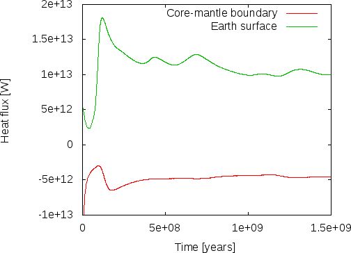
boundaries of our shell geometry. This is shown in the left panel of Fig. 40 where we plot the heat flux through
boundaries zero and one, corresponding to the core-mantle boundary and Earth’s surface. ASPECT always
computes heat fluxes in outward direction, so the flux through boundary zero will be negative, indicating the we
have a net flux into the mantle as expected. The figure indicates that after some initial jitters, heat flux from the
core to the mantle stabilizes at around 4.5 TW and that through the surface at around 10 TW, the difference of
5.5 TW resulting from the overall cooling of the mantle. While we cannot expect our model to be
quantitatively correct, this can be compared with estimates heat fluxes of 5–15 TW for the core-mantle
boundary, and an estimated heat loss due to cooling of the mantle of 7–15 TW (values again taken from
Wikipedia).
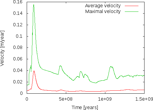
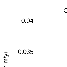
A second measure of whether these results make sense is to compare velocities in the mantle with what is known
from observations. As shown in the right panel of Fig. 40, the maximal velocities settle to values on the order of 3
cm/year (each of the peaks in the line for the maximal velocity corresponds to a particularly large
plume rising or falling). This is, again, at least not very far from what we know to be correct and
we should expect that with a more elaborate material model we should be able to get even closer to
reality.
5.3.3 Postprocessing spherical 3D convection
This section was contributed by Jacqueline Austermann, Ian Rose, and Shangxin Liu
There are several postprocessors that can be used to turn the velocity and pressure solution into quantities that
can be compared to surface observations. In this cookbook (cookbooks/shell_3d_postprocess.prm) we introduce
two postprocessors: dynamic topography and the geoid. We initialize the model with a harmonic perturbation of
degree 4 and order 2 and calculate the instantaneous solution. Analogous to the previous setup we use a spherical
shell geometry model and a simple material model.
The relevant section in the input file that determines the postprocessed output is as follows:
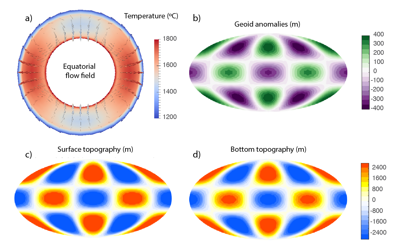
This initial condition results in distinct flow cells that cause local up- and downwellings (Figure 41). This flow
deflects the top and bottom boundaries of the mantle away from their reference height, a process known as
dynamic topography. The deflection of the surfaces and density perturbations within the mantle also
cause a perturbation in the gravitational field of the planet relative to the hydrostatic equilibrium
ellipsoid.
Dynamic topography at the surface and core mantle boundary.
Dynamic topography is calculated at the surface and bottom of the domain through a stress balancing approach
where we assume that the radial stress at the surface is balanced by excess (or deficit) topography. We use the
consistent boundary flux (CBF) method to calculate the radial stress at the surface [ZGH93]. For the
bottom surface we define positive values as up (out) and negative values are down (in), analogous to
the deformation of the upper surface. Dynamic topography can be outputted in text format (which
writes the Euclidean coordinates followed by the corresponding topography value) or as part of the
visualization. The upwelling and downwelling flow along the equator causes alternating topography high
and lows at the top and bottom surface (Figure 41). In Figure 41 c, d we have subtracted the mean
dynamic topography from the output field as a postproceesing step outside of Aspect. Since mass
is conserved within the Earth, the mean dynamic topography should always be zero, however, the
outputted values might not fullfill this constraint if the resolution of the model is not high enough
to provide an accurate solution. This cookbook only uses a refinement of 2, which is relatively low
resolution.
Geoid anomalies.
Geoid anomalies are perturbations of the gravitational equipotential surface that are due to density variations
within the mantle as well as deflections of the surface and core mantle boundary. The geoid anomalies are calculated
using a spherical harmonic expansion of the respective fields. The user has the option to specify the minimum
and maximum degree of this expansion. By default, the minimum degree is 2, which conserves the
mass of the Earth (by removing degree 0) and chooses the Earth’s center of mass as reference frame
(by removing degree 1). In this model, downwellings coincide with lows in the geoid anomaly. That
means the mass deficit caused by the depression at the surface is not fully compensated by the high
density material below the depression that drags the surface down. The geoid postprocessor uses a
spherical harmonic expansion and can therefore only be used with the 3D spherical shell geometry
model.
5.3.4 3D convection with an Earth-like initial condition
This section was contributed by Jacqueline Austermann
For any model run with ASPECT we have to choose an initial condition for the temperature field. If we
want to model convection in the Earth’s mantle we want to choose an initial temperature distribution
that captures the Earth’s buoyancy structure. In this cookbook we present how to use temperature
perturbations based on the shear wave velocity model S20RTS [RvH00] to initialize a mantle convection
calculation.
The input shear wave model.
The current version of ASPECT can read in the shear wave velocity models S20RTS [RvH00] and S40RTS
[RDvHW11], which are located in data/initial-_conditions/S40RTS/. Those models provide spherical harmonic
coefficients up do degree 20 and 40, respectively, for 21 depth layers. The interpolation with depth is done
through a cubic spline interpolation. The input files S20RTS.sph and S40RTS.sph were downloaded from
http://www.earth.lsa.umich.edu/~jritsema/Research.html and have the following format (this example is
S20RTS):
The first number in the first line denotes the maximum degree. This is followed in the next line by the spherical
harmonic coefficients from the surface down to the CMB. The coefficients are arranged in the following
way:
...
is the cosine
coefficient of degree
and order and
is the sine
coefficient of degree
and order .
The depth layers are specified in the file Spline_knots.txt by a normalized depth value ranging from the CMB
(3480km, normalized to -1) to the Moho (6346km, normalized to 1). This is the original format provided on the
homepage.
Any other perturbation model in this same format can also be used, one only has to specify the different filename
in the parameter file (see next section). For models with different depth layers one has to adjust the
Spline_knots.txt file as well as the number of depth layers, which is hard coded in the current code. A further
note of caution when switching to a different input model concerns the normalization of the spherical
harmonics, which might differ. After reading in the shear wave velocity perturbation one has several
options to scale this into temperature differences, which are then used to initialize the temperature
field.
Setting up the ASPECT model.
For this cookbook we will use the parameter file provided in cookbooks/S20RTS.prm, which uses a 3d spherical
shell geometry similar to section 5.3.2. This plugin is only sensible for a 3D spherical shell with Earth-like
dimensions.
The relevant section in the input file is as follows:
For this initial condition model we need to first specify the data directory in which the input files are located as
well as the initial condition file (S20RTS.sph or S40RTS.sph) and the file that contains the normalized depth layers
(Spline knots depth file name). We next have the option to remove the degree 0 perturbation from the shear wave
model. This might be the case if we want to make sure that the depth average temperature follows the background
(adiabatic or constant) temperature.
The next input parameters describe the scaling from the shear wave velocity
perturbation to the final temperature field. The shear wave velocity perturbation
(that is provided by S20RTS) is
scaled into a density perturbation
with a constant that is specified in the initial condition section of the input parameter file as ‘Vs to density scaling’.
Here we choose a constant scaling of 0.15. This perturbation is further translated into a temperature difference
by
multiplying it by the negative inverse of thermal expansion, which is also specified in this section of the parameter
file as ‘Thermal expansion coefficient in initial temperature scaling’. This temperature difference is then added to the
background temperature, which is the adiabatic temperature for a compressible model or the reference
temperature (as specified in this section of the parameter file) for an incompressible model. Features in the
upper mantle such as cratons might be chemically buoyant and therefore isostatically compensated, in
which case their shear wave perturbation would not contribute buoyancy variations. We therefore
included an additional option to zero out temperature perturbations within a certain depth, however,
in this example we don’t make use of this functionality. The chemical variation within the mantle
might require a more sophisticated ‘Vs to density’ scaling that varies for example with depth or as a
function of the perturbation itself, which is not captured in this model. The described procedure provides
an absolute temperature for every point, which will only be adjusted at the boundaries if indicated
in the Boundary temperature model. In this example we chose a surface and core mantle boundary
temperature that differ from the reference mantle temperature in order to approximate thermal boundary
layers.
Visualizing 3D models.
In this cookbook we calculate the instantaneous solution to examine the flow field. Figures 42 and 43 show some
of the output for a resolution of 2 global refinement steps (42c and 43a, c, e) as used in the cookbook, as well as 4
global refinement steps (other panels in these figures). Computations with 4 global refinements are expensive, and
consequently this is not the default for this cookbook. For example, as of 2017, it takes 64 cores approximately 2
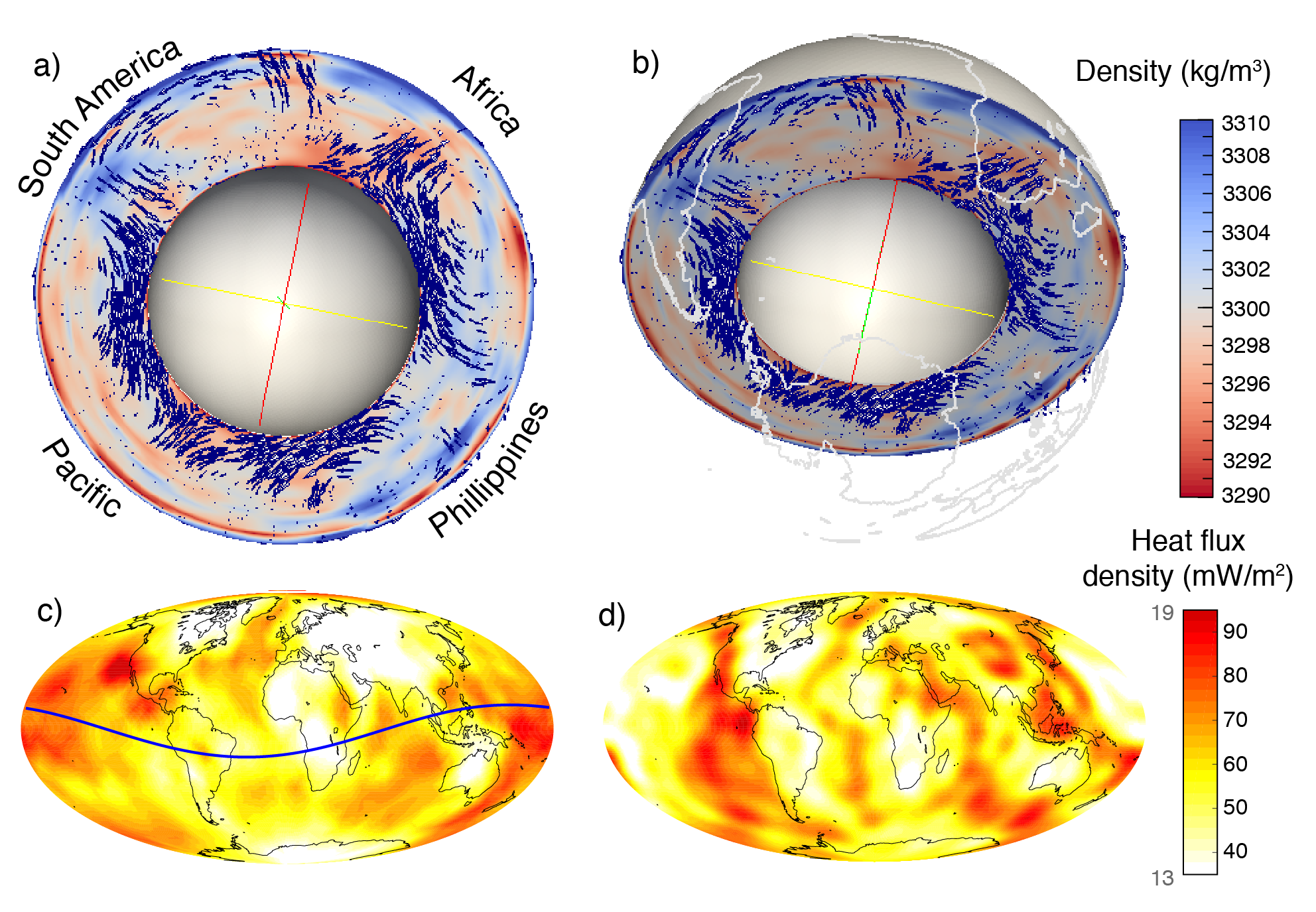
hours of walltime to finish this cookbook with 4 global refinements. Figure 42a and b shows the density
variation that has been obtained from scaling S20RTS in the way described above. One can see the
two large low shear wave velocity provinces underneath Africa and the Pacific that lead to upwelling
if they are assumed to be buoyant (as is done in this case). One can also see the subducting slabs
underneath South America and the Philippine region that lead to local downwelling. Figure 42c and d
shows the heat flux density at the surface for 2 refinement steps (c, colorbar ranges from 13 to 19
mW/) and for 4 refinement steps (d,
colorbar ranges from 35 to 95 mW/).
A first order correlation with upper mantle features such as high heat flow at mid ocean ridges and low heat flow at
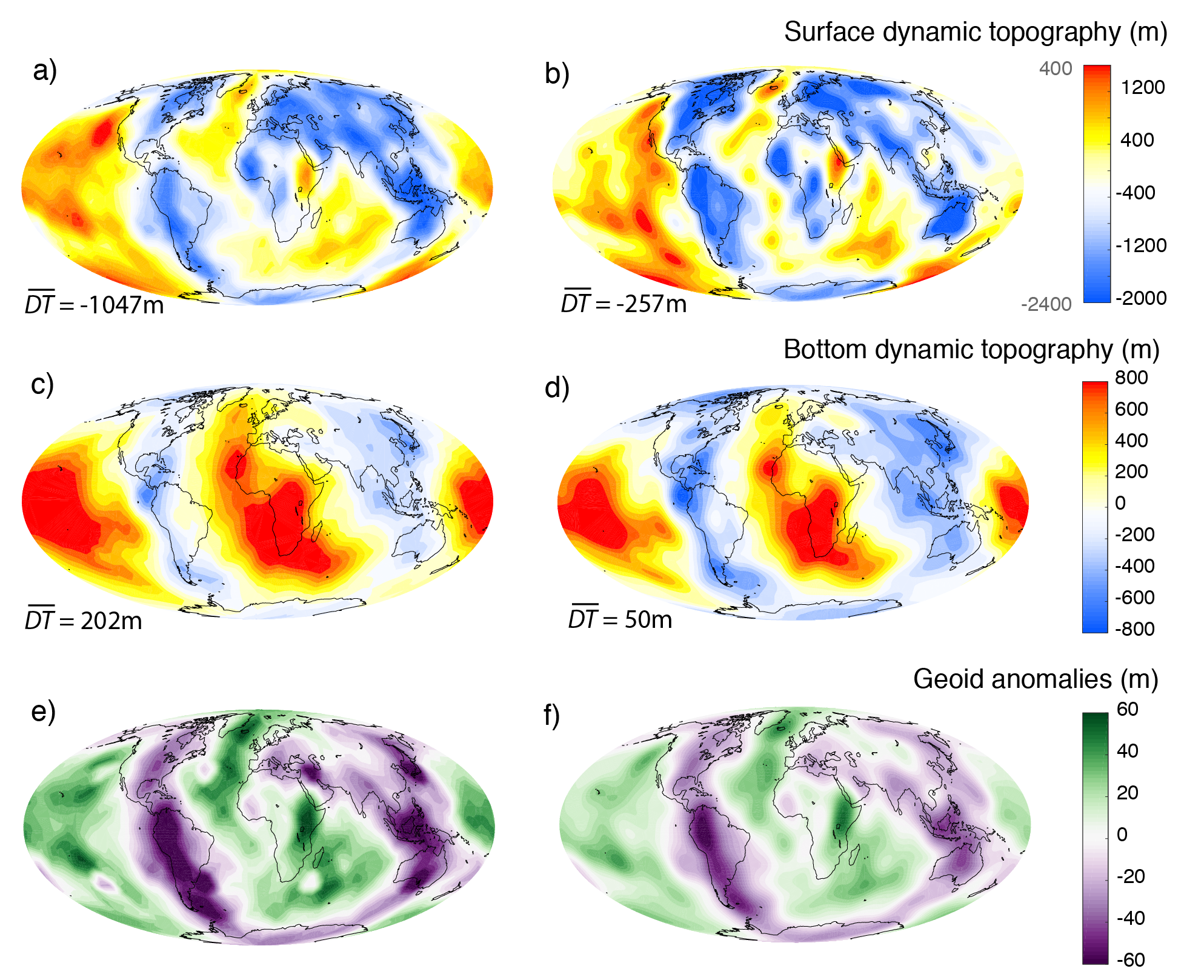
cratons is correctly initialized by the tomography model. The mantle flow and bouyancy variations produce dynamic
topography on the top and bottom surface, which is shown for 2 refinement steps (43a and c, respectively) and 4
refinement steps (43b and d, respectively). One can see that subduction zones are visible as depressed surface
topography due to the downward flow, while regions such as Iceland, Hawaii, or mid ocean ridges are elevated due to
(deep and) shallow upward flow. The core mantle boundary topography shows that the upwelling large low shear
wave velocity provinces deflect the core mantle boundary up. Lastly, Figure 43e and f show geoid
perturbations for 2 and 4 global refinement steps, respectively. The geoid anomalies show a strong correlation
with the surface dynamic topography. This is in part expected given that the geoid anomalies are
driven by the deflection of the upper and lower surface as well as internal density variations. The
relative importance of these different contributors is dictated by the Earth’s viscosity profile. Due
to the isoviscous assumption in this cookbook, we don’t properly recover patterns of the observed
geoid.
As discussed in the previous cookbook, dynamic topography does not necessarily average to zero if the resolution
is not high enough. While one can simply subtract the mean as a postprocessing step this should be done with
caution since a non-zero mean indicates that the refinement is not sufficiently high to resolve the convective flow. In
Figure 43a-d we refrained from subtracting the mean but indicated it at the bottom left of each panel. The mean
dynamic topography approaches zero for increasing refinement. Furthermore, the mean bottom dynamic topography
is closer to zero than the mean top dynamic topography. This is likely due to the larger magnitude of dynamic
topography at the surface and the difference in resolution between the top and bottom domain (for a given
refinement, the resolution at the core mantle boundary is higher than the resolution at the surface).
The average geoid height is zero since the minimum degree in the geoid anomaly expansion is set to
2.
This model uses a highly simplified material model that is incompressible and isoviscous and does therefore not
represent real mantle flow. More realistic material properties, density scaling as well as boundary conditions will
affect the magnitudes and patterns shown here.
5.3.5 Using reconstructed surface velocities by GPlates
This section was contributed by René Gaßmöller
In a number of model setups one may want to include a surface velocity boundary condition that prescribes the
velocity according to a specific geologic reconstruction. The purpose of this kind of models is often to test a
proposed geologic model and compare characteristic convection results to present-day observables in
order to gain information about the initially assumed geologic input. In this cookbook we present
ASPECT’s interface to the widely used plate reconstruction software GPlates, and the steps to go from
a geologic plate reconstruction to a geodynamic model incorporating these velocities as boundary
condition.
Acquiring a plate reconstruction.
The plate reconstruction that is used in this cookbook is included in the data/velocity-boundary-conditions/gplates/
directory of your ASPECT installation. For a new model setup however, a user eventually needs to create her own
data files, and so we will briefly discuss the process of acquiring a usable plate reconstruction and transferring it into
a format usable by ASPECT. Both the necessary software and data are provided by the GPlates
project. GPlates is an open-source software for interactive visualization of plate tectonics. It is developed
by the EarthByte Project in the School of Geosciences at the University of Sydney, the Division of
Geological and Planetary Sciences (GPS) at CalTech and the Center for Geodynamics at the Norwegian
Geological Survey (NGU). For extensive documentation and support we refer to the GPlates website
(http://www.gplates.org). Apart from the software one needs the actual plate reconstruction that consists of
closed polygons covering the complete model domain. For our case we will use the data provided by
[GTZ12] that is available from the
GPlates website under “Download
Download GPlates-compatible data
Global reconstructions with continuously closing plates from 140 Ma to the present”. The data is provided under a
Creative Commons Attribution 3.0 Unported License (http://creativecommons.org/licenses/by/3.0/).
Converting GPlates data to ASPECT input.
After loading the data files into GPlates (*.gpml for plate polygons, *.rot for plate rotations over time) the user
needs to convert the GPlates data to velocity information usable in ASPECT. The purpose of this step is to
convert from the description GPlates uses internally (namely a representation of plates as polygons that rotate with
a particular velocity around a pole) to one that can be used by ASPECT (which needs velocity vectors defined at
individual points at the surface).
With loaded plate polygon and rotation information the conversion from GPlates data to ASPECT-readable velocity
files is rather straightforward. First the user needs to generate (or import) so-called “velocity domain points”, which
are discrete sets of points at which GPlates will evaluate velocity information. This is done using the “Features
Generate Velocity
Domain Points
Latitude Longitude” menu option. Because ASPECT is using an adaptive mesh it is not possible for GPlates to
generate velocity information at the precise surface node positions like for CitcomS or Terra (the other currently
available interfaces). Instead GPlates will output the information on a general Latitude/Longitude grid with nodes
on all crossing points. ASPECT then internally interpolates this information to the current node locations during
the model run. This requires the user to choose a sensible resolution of the GPlates output, which can be adjusted in
the “Generate Latitude/Longitude Velocity Domain Points” dialog of GPlates. In general a resolution that resolves
the important features is necessary, while a resolution that is higher than the maximal mesh size for the
ASPECT model is unnecessary and only increases the computational cost and memory consumption of the
model.
Important note: The Mesh creation routine in GPlates has significantly changed from version 1.3 to 1.4. In
GPlates 1.4 and later the user has to make sure that the number of longitude intervals is set as twice
the number of latitude intervals, the “Place node points at centre of latitude/longitude cells” box is
unchecked and the “Latitude/Longitude extents” are set to “Use Global Extents”. ASPECT does
check for most possible combinations that can not be read and will cancel the calculation in these
cases, however some mistakes can not be checked against from the information provided in the GPlates
file.
After creating the Velocity Domain Points the user should see the created points and their velocities indicated as
points and arrows in GPlates. To export the calculated velocities one would use the “Reconstruction
Export”
menu. In this dialog the user may specify the time instant or range at which the velocities shall be exported. The
only necessary option is to include the “Velocities” data type in the “Add Export” sub-dialog. The velocities need to
be exported in the native GPlates *.gpml format, which is based on XML and can be read by ASPECT. In case of
a time-range the user needs to add a pattern specifier to the name to create a series of files. The %u flag is especially
suited for the interaction with ASPECT, since it can easily be replaced by a calculated file index (see also
5.3.5).
Setting up the ASPECT model.
For this cookbook we will use the parameter file provided in cookbooks/gplates-_2d.prm which uses the 2d
shell geometry previously discussed in Section 5.3.1. ASPECT’s GPlates plugin allows for the use of two- and
three-dimensional models incorporating the GPlates velocities. Since the output by GPlates is three-dimensional in
any case, ASPECT internally handles the 2D model by rotating the model plane to the orientation specified by the
user and projecting the plate velocities into this plane. The user specifies the orientation of the model plane
by prescribing two points that define a plane together with the coordinate origin (i.e. in the current
formulation only great-circle slices are allowed). The coordinates need to be in spherical coordinates
and
with
being the colatitude
(0 at north pole) and
being the longitude (0 at Greenwich meridian, positive eastwards) both given in radians. The approach of
identifying two points on the surface of the Earth along with its center allows to run computations on arbitrary
two-dimensional slices through the Earth with realistic boundary conditions.
The relevant section of the input file is then as follows:
In the “Boundary velocity model” subsection the user prescribes the boundary that is supposed to use the
GPlates plugin. Although currently nothing forbids the user to use GPlates plugin for other boundaries than the
surface, its current usage and the provided sample data only make sense for the surface of a spherical
shell (boundary number 1 in the above provided parameter file). In case you are familiar with this
kind of modeling and the plugin you could however also use it to prescribe mantle movements below a
lithosphere model. All plugin specific options may be set in section ??. Possible options include the data
directory and file name of the velocity file/files, the time step (in model units, mostly seconds or years
depending on the “Use years in output instead of seconds” flag) and the points that define the
2D plane. The parameter “Interpolation width” is used to smooth the provided velocity files by
a moving average filter. All velocity data points within this distance are averaged to determine the
actual boundary velocity at a certain mesh point. This parameter is usually set to 0 (no interpolation,
use nearest velocity point data) and is only needed in case the original setting is unstable or slowly
converging.
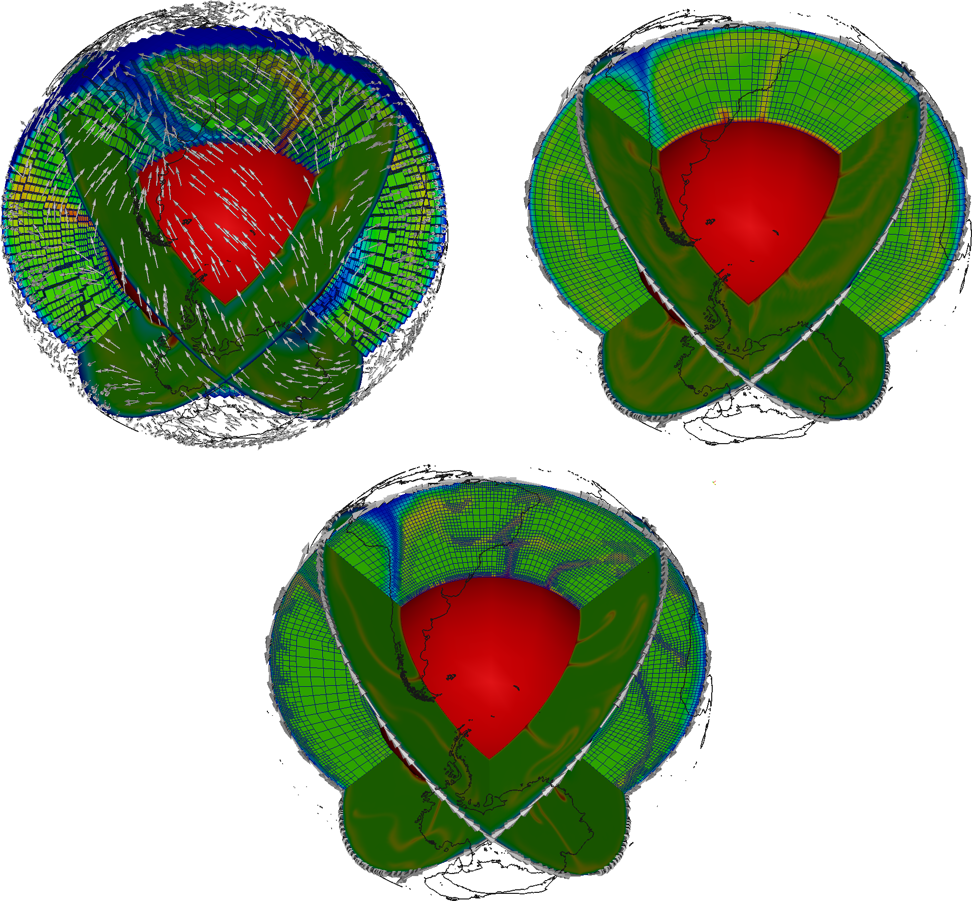
Comparing and visualizing 2D and 3D models.
The implementation of plate velocities in both two- and three-dimensional model setups allows for an easy
comparison and test for common sources of error in the interpretation of model results. The left top figure in Fig. 44
shows a modification of the above presented parameter file by setting “Dimension = 3” and “Initial global
refinement = 3”. The top right plot of Fig. 44 shows an example of three independent two-dimensional
computations of the same reduced resolution. The models were prescribed to be orthogonal slices by
setting:
and
The results of these models are plotted simultaneously in a single three-dimensional figure in their respective
model planes. The necessary information to rotate the 2D models to their respective planes (rotation axis and angle)
is provided by the GPlates plugin in the beginning of the model output. The bottom plot of Fig. 44
finally shows the results of the original cookbooks/gplates-_2d.prm also in the three mentioned
planes.
Now that we have model output for otherwise identical 2D and 3D models with equal resolution and additional
2D output for a higher resolution an interesting question to ask would be: What additional information can be
created by either using three-dimensional geometry or higher resolution in mantle convection models with prescribed
boundary velocities. As one can see in the comparison between the top right and bottom plot in Fig. 44 additional
resolution clearly improves the geometry of small scale features like the shape of up- and downwellings as well as the
maximal temperature deviation from the background mantle. However, the limitation to two dimensions leads to
inconsistencies, that are especially apparent at the cutting lines of the individual 2D models. Note for example
that the Nacza slab of the South American subduction zone is only present in the equatorial model
plane and is not captured in the polar model plane west of the South American coastline. The (coarse)
three-dimensional model on the other hand shows the same location of up- and downwellings but
additionally provides a consistent solution that is different from the two dimensional setups. Note that the
Nazca slab is subducting eastward, while all 2D models (even in high resolution) predict a westward
subduction.
Finally we would like to emphasize that these models (especially the used material model) are way too simplified
to draw any scientific conclusion out of it. Rather it is thought as a proof-of-concept what is possible with the
dimension independent approach of ASPECT and its plugins.
Time-dependent boundary conditions.
The example presented above uses a constant velocity boundary field that equals the present day plate
movements. For a number of purposes one may want to use a prescribed velocity boundary condition that changes
over time, for example to investigate the effect of trench migration on subduction. Therefore ASPECT’s GPlates
plugin is able to read in multiple velocity files and linearly interpolate between pairs of files to the current model
time. To achieve this, one needs to use the %d wildcard in the velocity file name, which represents the current
velocity file index (e.g. time_dependent.%d.gpml). This index is calculated by dividing the current model time
by the user-defined time step between velocity files (see parameter file above). As the model time
progresses the plugin will update the interpolation accordingly and if necessary read in new velocity
files. In case it can not read the next velocity file, it assumes the last velocity file to be the constant
boundary condition until the end of the model run. One can test this behavior with the provided data files
data/velocity_boundary_conditions/gplates/time_dependent.%d.gpml with the index d ranging from
0 to 3 and representing the plate movements of the last 3 million years corresponding to the same
plate reconstruction as used above. Additionally, the parameter Velocity file start time allows
for a period of no-slip boundary conditions before starting the use of the GPlates plugin. This is a
comfort implementation, which could also be achieved by using the checkpointing possibility described in
section 4.5.
5.3.6 2D compressible convection with a reference profile and material properties from BurnMan
This section was contributed by Juliane Dannberg and René Gassmöller
In this cookbook we will set up a compressible mantle convection model that uses the (truncated) anelastic
liquid approximation (see Sections 2.10.1 and 2.10.2), together with a reference profile read in from an ASCII
data file. The data we use here is generated with the open source mineral physics toolkit BurnMan
(http://www.burnman.org) using the python example program simple_adiabat.py. This file is available as a part
of BurnMan, and provides a tutorial for how to generate ASCII data files that can be used together with ASPECT.
The computation is based on the Birch-Murnaghan equation of state, and uses a harzburgitic composition. However,
in principle, other compositions or equations of state can be used, as long as the reference profile contains data for
the reference temperature, pressure, density, gravity, thermal expansivity, specific heat capacity and
compressibility. Using BurnMan to generate the reference profile has the advantage that all the material
property data are consistent, for example, the gravity profile is computed using the reference density.
The reference profile is shown in Figure 45, and the corresponding data file is located at
data/adiabatic-_conditions/ascii-_data/isentrope_properties.txt.
Setting up the ASPECT model.
In order to use this profile, we have to import and use the data in the adiabatic conditions model, in the gravity
model and in the material model, which is done using the corresponding ASCII data plugins. The input file is
provided in cookbooks/burnman.prm, and it uses the 2d shell geometry previously discussed in Section 5.3.1 and
surface velocities imported from GPlates as explained in Section 5.3.5.
To use the BurnMan data in the material model, we have to specify that we want to use the ascii reference
profile model. This material model makes use of the functionality provided by the AsciiData classes in
ASPECT, which allow plugins such as material models, boundary or initial conditions models to read in ASCII
data files (see for example Section 5.2.12). Hence, we have to provide the directory and file name of the data to be
used in the separate subsection Ascii data model, and the same functionality and syntax will also be used for the
adiabatic conditions and gravity model.
The viscosity in this model is computed as the product of a profile
, where
corresponds to the depth direction of the chosen geometry model, and a term that describes the dependence on
temperature:
where
and are
constants determined in the input file via the parameters Viscosity and Thermal viscosity exponent, and
is a
stepwise constant function that determines the viscosity profile. This function can be specified by
providing a list of Viscosity prefactors and a list of depths that describe in which depth range each
prefactor should be applied, in other words, at which depth the viscosity changes. By default, it is set to
viscosity jumps at 150 km depth, between upper mantle and transition zone, and between transition
zone and lower mantle). The prefactors used here lead to a low-viscosity asthenosphere, and high
viscosities in the lower mantle. To make sure that these viscosity jumps do not lead to numerical problems
in our computation (see Section 5.2.8), we also use harmonic averaging of the material properties.
As the reference profile has a depth dependent density and also contains data for the compressibility, this material
model supports compressible convection models.
For the adiabatic conditions and the gravity model, we also specify that we want to use the respective ascii
data plugin, and provide the data directory in the same way as for the material model. The gravity model
automatically uses the same file as the adiabatic conditions model.
To make use of the reference state we just imported from BurnMan, we choose a formulation of the equations
that employs a reference state and compressible convection, in this case the anelastic liquid approximation (see
Section 2.10.1).
This means that the reference profiles are used for all material properties in the model, except for the density in the
buoyancy term (on the right-hand side of the force balance equation (1), which in the limit of the anelastic liquid
approximation becomes Equation (21)). In addition, the density derivative in the mass conservation equation (see
Section 2.11.1) is taken from the adiabatic conditions, where it is computed as the depth derivative of the provided
reference density profile (see also Section 2.11.5).
Visualizing the model output.
If we look at the output of our model (for example in ParaView), we can see how cold, highly viscous slabs are
subducted and hot plumes rise from the core-mantle boundary. The final time step of the model is shown in
Figure 46, and the full model evolution can be found at https://youtu.be/nRBOpw5kp-_4. Visualizing material
properties such as density, thermal expansivity or specific heat shows how they change with depth, and
reveals abrupt jumps at the phase transitions, where properties change from one mineral phase to the
next. We can also visualize the gravity and the adiabatic profile, to ensure that the data we provided
in the data/adiabatic-_conditions/ascii-_data/isentrope_properties.txt file is used in our
model.
Comparing different model approximations.
For the model described above, we have used the anelastic liquid approximation. However, one might
want to use different approximations that employ a reference state, such as the truncated anelastic
liquid approximation (TALA, see Section 2.10.2), which is also supported by the ascii reference
profile material model. In this case, the only change compared to ALA is in the density used in
the buoyancy term, the only place where the temperature-dependent density instead of the reference
density is used. For the TALA, this density only depends on the temperature (and not on the dynamic
pressure, as in the ALA). Hence, we have to make this change in the appropriate place in the material
model (while keeping the formulation of the equations set to anelastic liquid approximation):
We now want to compare these commonly used approximations to the “isothermal compression approximation”
(see Section 2.10.4) that is unique to ASPECT. It does not require a reference state and uses the full density
everywhere in the equations except for the right-hand side mass conservation, where the compressibility is used to
compute the density derivative with regard to pressure. Nevertheless, this formulation can make use of the reference
profile computed by BurnMan and compute the dependence of material properties on temperature and pressure in
addition to that by taking into account deviations from the reference profile in both temperature and
pressure. As this requires a modification of the equations outside of the material model, we have to
specify this change in the Formulation (and remove the lines for the use of TALA discussed above).
As the “isothermal compression approximation” is also ASPECT’s default for compressible models, the same
model setup can also be achieved by just removing the lines that specify which Formulation should be
used.
The Figures 47 and 48 show a comparison between the different models. They demonstrate that upwellings and
downwellings may occur in slightly different places and at slightly different times when using a different
approximation, but averaged model properties describing the state of the model – such as the root mean square
velocity – are similar between the models.
5.3.7 Reproducing rheology of Morency and Doin, 2004
This section was contributed by Jonathan Perry-Houts
Modeling interactions between the upper mantle and the lithosphere can be difficult because of the dynamic
range of temperatures and pressures involved. Many simple material models will assign very high viscosities at low
temperature thermal boundary layers. The pseudo-brittle rheology described in [MD04] was developed to limit the
strength of lithosphere at low temperature. The effective viscosity can be described as the harmonic mean of two
non-Newtonian rheologies:
where
where is a
scaling constant;
is defined as the quadratic sum of the second invariant of the strain rate tensor and a minimum strain rate,
;
is a reference
strain rate; , and
are stress exponents;
is the activation energy;
is the activation
volume; is the mantle
density; is the gas
constant; is temperature;
is the cohesive strength of rocks at
the surface; is a coefficient of yield
stress increase with depth; and
is depth.
By limiting the strength of the lithosphere at low temperature, this rheology allows one to more realistically
model processes like lithospheric delamination and foundering in the presence of weak crustal layers. A
similar model setup to the one described in [MD04] can be reproduced with the files in the directory
cookbooks/morency_doin_2004. In particular, the following sections of the input file are important to reproduce
the setup:
Note: [MD04] defines the second invariant of the strain rate in
a nonstandard way. The formulation in the paper is given as
,
where
is the strain rate tensor. For consistency, that is also the formulation implemented in
ASPECT.
Because of this irregularity it is inadvisable to use this material model for purposes beyond
reproducing published results.
Note: The viscosity profile in Figure 1 of
[MD04] appears to be wrong. The published parameters
do not reproduce those viscosities; it is unclear why. The values used here get very close. See
Figure
49 for an approximate reproduction of the original figure.
5.3.8 Crustal deformation
This section was contributed by Cedric Thieulot, and makes use of the Drucker-Prager material model written by
Anne Glerum and the free surface plugin by Ian Rose.
This is a simple example of an upper-crust undergoing compression or extension. It is characterized by a single
layer of visco-plastic material subjected to basal kinematical boundary conditions. In compression, this setup is
somewhat analogous to [Wil99], and in extension to [AHT11].
Brittle failure is approximated by adapting the viscosity to limit the stress that is generated during deformation.
This “cap” on the stress level is parameterized in this experiment by the pressure-dependent Drucker Prager yield
criterion and we therefore make use of the Drucker-Prager material model (see Section ??) in the
cookbooks/crustal_model_2D.prm.
The layer is assumed to have dimensions of 80km
16km and to
have a density
kg/m.
The plasticity parameters are specified as follows:
The yield strength
is a function of pressure, cohesion and angle of friction (see Drucker-Prager material model in Section ??), and the
effective viscosity is then computed as follows:
where
is the square root of the second invariant of the deviatoric strain rate. The viscosity cutoffs insure that the viscosity
remains within computationally acceptable values.
During the first iteration of the first timestep, the strain rate is zero, so we avoid dividing by zero by setting the
strain rate to Reference strain rate.
The top boundary is a free surface while the left, right and bottom boundaries are subjected to the following
boundary conditions:
Note that compressive boundary conditions are simply achieved by reversing the sign of the imposed
velocity.
The free surface will be advected up and down according to the solution of the Stokes solve. We have a choice
whether to advect the free surface in the direction of the surface normal or in the direction of the local vertical
(i.e., in the direction of gravity). For small deformations, these directions are almost the same, but in
this example the deformations are quite large. We have found that when the deformation is large,
advecting the surface vertically results in a better behaved mesh, so we set the following in the free surface
subsection:
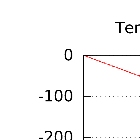
We also make use of the strain rate-based mesh refinement plugin:
Setting set Initial adaptive refinement = 4 yields a series of meshes as shown in Fig. (50), all produced
during the first timestep. As expected, we see that the location of the highest mesh refinement corresponds to the
location of a set of conjugated shear bands.
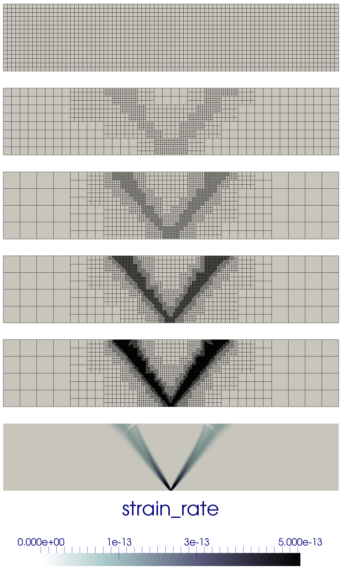
If we now set this parameter to 1 and allow the simulation to evolve for 500kyr, a central graben or plateau
(depending on the nature of the boundary conditions) develops and deepens/thickens over time, nicely showcasing
the unique capabilities of the code to handle free surface large deformation, localised strain rates through
visco-plasticity and adaptive mesh refinement as shown in Fig. (51).
Deformation localizes at the basal velocity discontinuity and plastic shear bands form at an angle of approximately
to the bottom in
extension and
in compression, both of which correspond to the reported Arthur angle [Kau10, Bui12].
Extension to 3D.
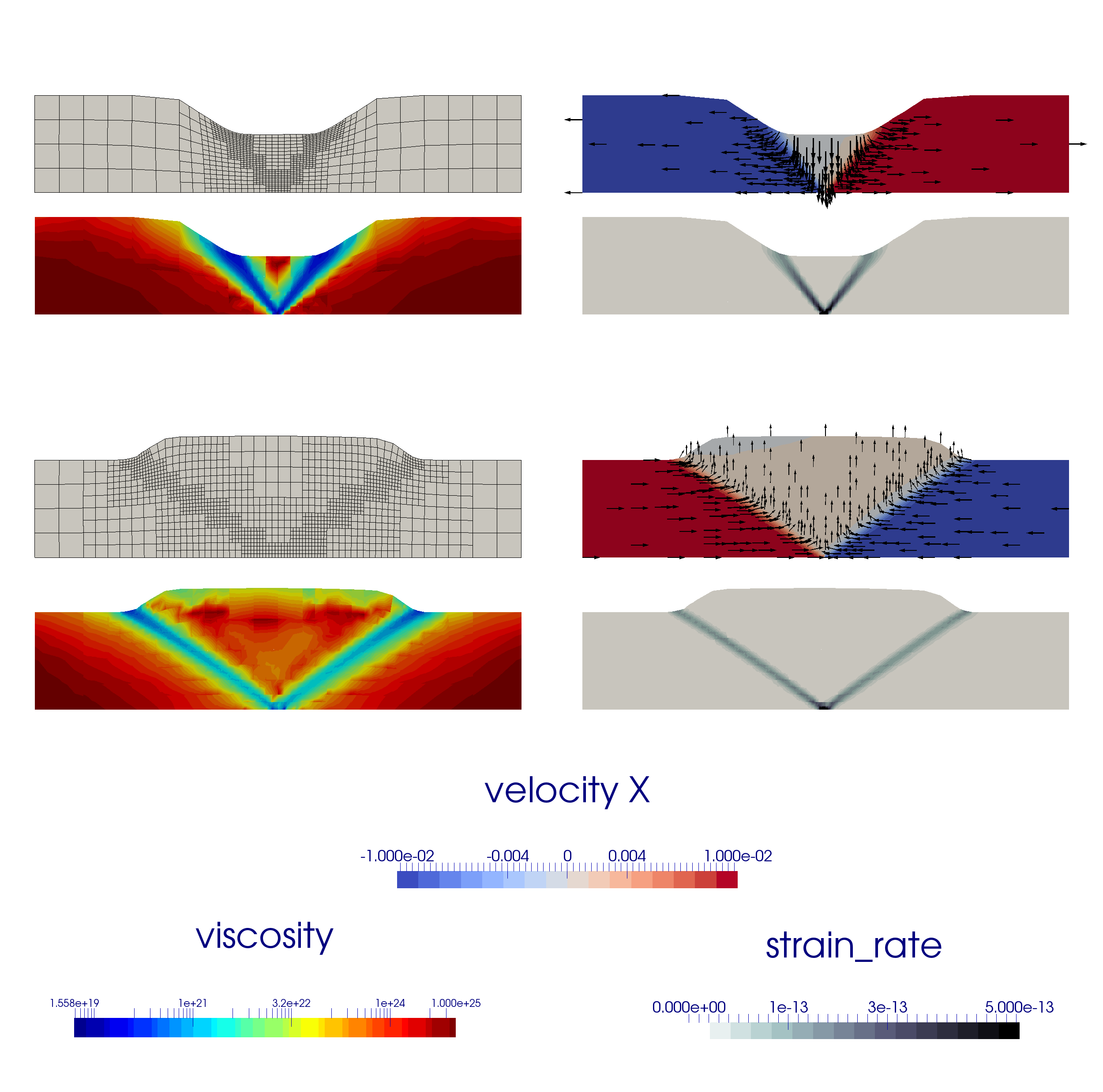
We can easily modify the previous input file to produce crustal_model_3D.prm which implements a similar
setup, with the additional constraint that the position of the velocity discontinuity varies with the
-coordinate, as shown in Fig.
(52). The domain is now km
and the boundary conditions are implemented as follows:
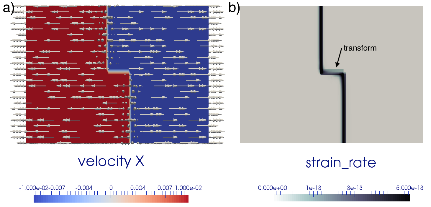
The presence of an offset between the two velocity discontinuity zones leads to a transform fault which connects
them.
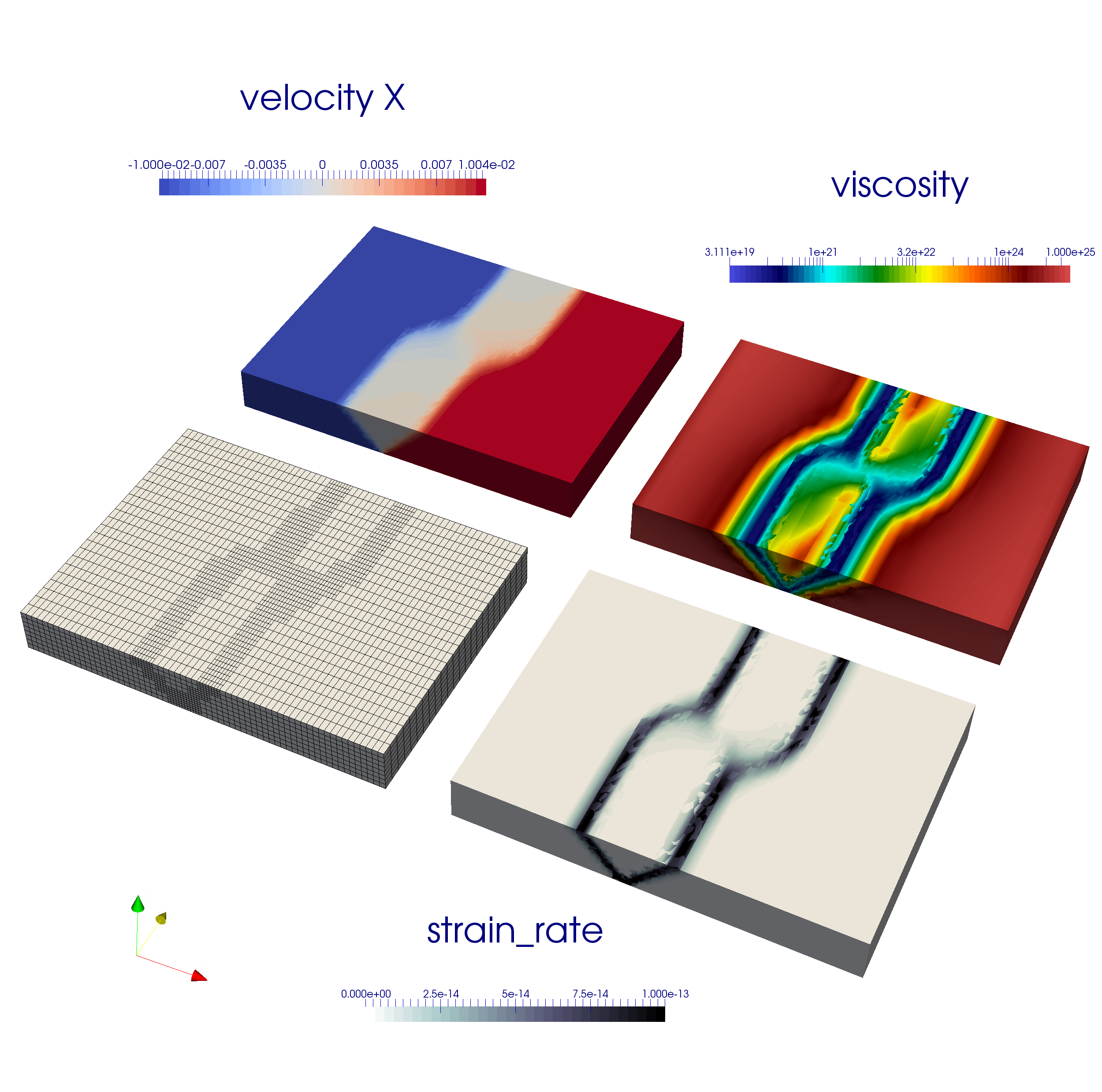
The Finite Element mesh, the velocity, viscosity and strain rate fields are shown in Fig. (53) at the end of the
first time steps. The reader is encouraged to run this setup in time to look at how the two grabens interact as a
function of their initial offset [AHT11, AHT12, AHFT13].
5.3.9 Continental extension
This section was contributed by John Naliboff
In the crustal deformation examples above, the viscosity depends solely on the Drucker Prager yield criterion
defined by the cohesion and internal friction angle. While this approximation works reasonably well for the
uppermost crust, deeper portions of the lithosphere may undergo either brittle or viscous deformation, with the
latter depending on a combination of composition, temperature, pressure and strain-rate. In effect, a combination of
the Drucker-Prager and Diffusion dislocation material models is required. The visco-plastic material model is
designed to take into account both brittle (plastic) and non-linear viscous deformation, thus providing a template
for modeling complex lithospheric processes. Such a material model can be used in ASPECT using the following set
of input parameters:
This cookbook provides one such example where the continental lithosphere undergoes extension. Notably, the model
design follows that of numerous previously published continental extension studies [HB11, BHPeGeS14, NB15, and
references therein].
Continental Extension
The 2D Cartesian model spans 400 (x) by 100 (y) km and has a finite element grid with uniform 2 km
spacing. Unlike the crustal deformation cookbook (see Section 5.3.8, the mesh is not refined with
time.
Similar to the crustal deformation examples above, this model contains a free surface. Deformation is driven by constant horizontal
(-component) velocities (0.25 cm/yr)
on the side boundaries (-velocity
component unconstrained), while the bottom boundary has vertical inflow to balance the lateral outflow. The top,
and bottom boundaries have fixed temperatures, while the sides are insulating. The bottom boundary is also
assigned a fixed composition, while the top and sides are unconstrained.
Sections of the lithosphere with distinct properties are represented by compositional fields for the upper crust (20
km thick), lower crust (10 km thick) and mantle lithosphere (70 km thick). A mechanically weak seed within the
mantle lithosphere helps localize deformation. Material (viscous flow law parameters, cohesion, internal friction
angle) and thermodynamic properties for each compositional field are based largely on previous numerical studies.
Dislocation creep viscous flow parameters are taken from published deformation experiments for wet quartzite
[RB04], wet anorthite [RGWD06] and dry olivine [HK04].
The initial thermal structure, radiogenic heating model and associated thermal properties are consistent with the
prescribed thermal boundary conditions and produce a geotherm characteristic of the continental lithosphere. The
equations defining the initial geotherm [Cha86] follow the form
where T is temperature, z is depth, is the
temperature at the layer surface (top),
is surface heat flux, is
thermal conductivity, and
is radiogenic heat production.
For a layer thickness ,
the basal temperature ()
and heat flux ()
are
In this example, specifying the top (273 K) and bottom temperature (1573 K), thermal conductivity of each layer
and radiogenic heat production in each layer provides enough constraints to successively solve for the temperature
and heat flux at the top of the lower crust and mantle.
As noted above, the mechanically weak seed placed within the mantle localizes the majority of deformation onto
two conjugate shear bands that propagate from the surface of the seed to the free surface. After 5 million years of
extension background ‘stretching’ is clearly visible in the strain-rate field, but deformation is still largely focused
within the set of conjugate shear bands originating at the weak seed (Fig. 54). As expected, crustal thickness and
surface topography patterns reveal a relatively symmetric horst and graben structure, which arises from
displacements along the shear bands (Fig. 55). While deformation along the two major shear bands
dominates at this early stage of extension, additional shear bands often develop within the horst-graben
system leading to small inter-graben topographic variations. This pattern is illustrated in a model
with double the numerical resolution (initial 1 km grid spacing) after 10 million years of extension
(Fig. 56).
With further extension for millions of years, significant crustal thinning and surface topography development
should occur in response to displacement along the conjugate shear bands. However, given that the model only
extends to 100 km depth, the simulation will not produce a realistic representation of continental breakup due to the
lack of an upwelling asthenosphere layer. Indeed, numerical studies that examine continental breakup, rather than
just the initial stages of continental extension, include an asthenospheric layer or modified basal boundary
conditions (e.g. Winkler boundary condition [BHPeGeS14, for example]) as temperature variations
associated with lithospheric thinning exert a first-order influence on the deformation patterns. As
noted below, numerous additional parameters may also affect the temporal evolution of deformation
patterns.
Note: It is important to consider that the non-linearity of visco-plastic rheologies and
mesh-dependence of brittle shear bands make lithospheric deformation models highly sensitive
to a large number of parameters. In order to ensure the conclusions drawn from a series of
numerical experiments are robust, one should complete a sensitivity test for a large range of
parameters including grid resolution, model geometry, boundary conditions, initial composition
and temperature conditions, material properties, composition discretization, CFL number and
solver settings. If you are new to modeling lithospheric processes, a reasonable starting point is to
try and reproduce results from a relevant previous study and then perform a sensitivity test for
the parameters listed above. While highly time consuming, completing this procedure will prove
invaluable when you design and assess the results of your own numerical study.
5.3.10 Inner core convection
This section was contributed by Juliane Dannberg, and the model setup was inspired by discussions with John Rudge.
Additional materials and comments by Mathilde Kervazo and Marine Lasbleis.
This is an example of convection in the inner core of the Earth. The model is based on a spherical geometry,
with a single material. Three main particularities are constitutive of this inner core dynamics modeling: it
consists of a self-gravitating sphere where the gravity decreases linearly from the boundary to zero at the
center of the inner core; the boundary conditions combine normal stress and normal velocity, and
take into account the rate of phase change (melting/freezing) at the inner-outer core boundary; the
material has a temperature dependent density that makes the density profile unstably stratified as
temperature increases towards the center of the core. Note that we do not actually compute self-gravitation,
but instead define a linear gravity profile. Since the density variations are very small, this is a good
approximation.
The setup is analogous to the models described in [DAC13], and all material properties are chosen in a way so
that the equations are non-dimensional.
The required heating model and changes to the material model are implemented in a shared library
(cookbooks/inner_core_convection/inner_core_convection.cc).
In the non-dimensional form of the equations derived by [DAC13], we solve for the potential temperature
( is the
temperature field,
the isentropic – also called adiabatic – temperature). This allows to solve the temperature field with simple boundary
conditions (),
even if the temperature of the inner core boundary evolves with time, defined as the intersection between the
isentrope and the liquidus of the material in the outer core. The equations for inner core convection in the
approximation of no growth (equation 59 for the potential temperature) are
where is the Rayleigh
number and is
the ’source term’, constructed when removing the adiabatic temperature from the temperature field to obtain the potential
temperature .
describes
the time-evolution of the adiabatic temperature over time, due to secular cooling of the outer core. In spherical geometry,
.
Mechanical boundary. The mechanical boundary conditions for the inner core are
tangential stress-free and continuity of the normal stress at the inner-outer core boundary.
For the non-dimensional equations, that means that we define a “phase change number”
(see [DAC13]) so that the
normal stress at the boundary is
with the radial velocity .
This number characterizes the resistance to phase change at the boundary, with
corresponding to infinitely slow melting/freezing (or a free slip boundary), and
corresponding to instantaneous melting/freezing (or a zero normal stress, corresponding to an open
boundary).
In the weak form, this results in boundary conditions of the form of a surface integral:
with the normal vector .
This phase change term is added to the matrix in the cookbooks/inner_core_convection/inner_core_assembly.cc
plugin by using a signal (as described in Section 6.5). The signal connects the function set_assemblers_phase_boundary,
which is only called once at the beginning of the model run. It creates the new assembler PhaseBoundaryAssembler for
the boundary faces of the Stokes system and adds it to the list of assemblers executed in every time step. The assembler
contains the function phase_change_boundary_conditions that loops over all faces at the model boundary, queries the
value of
from the material model, and adds the surface integral given above to the matrix:
Instructions for how to compile and run models with a shared library are given in Section 5.4.1.
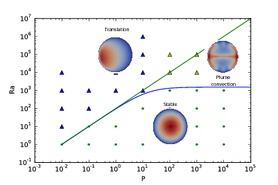
Governing parameters. Analyzing Equations (51)–(53), two parameters determine the dynamics of convection in the inner core:
the Rayleigh number and
the phase change number .
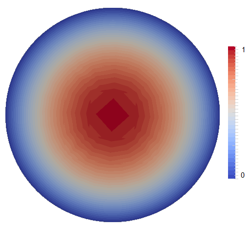
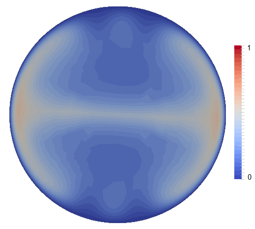
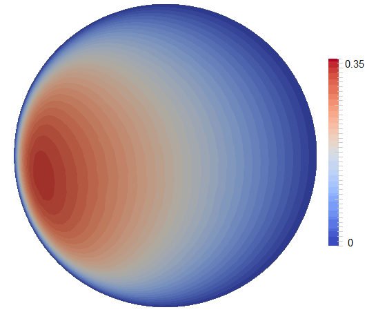
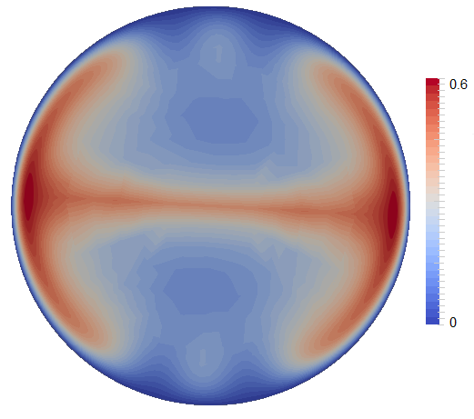
Three main areas can be distinguished: the stable area, the plume convection area and the
translation mode of convection area (Figure 57). For low Rayleigh numbers (below the critical value
), there is no
convection and thermal diffusion dominates the heat transport. However, if the inner core is convectively unstable
(>),
the convection regime depends mostly on .
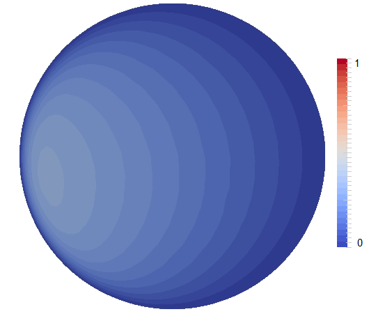
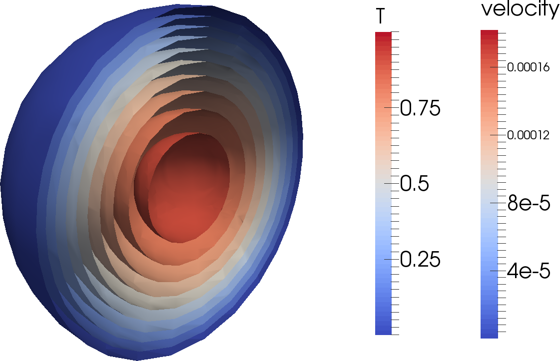
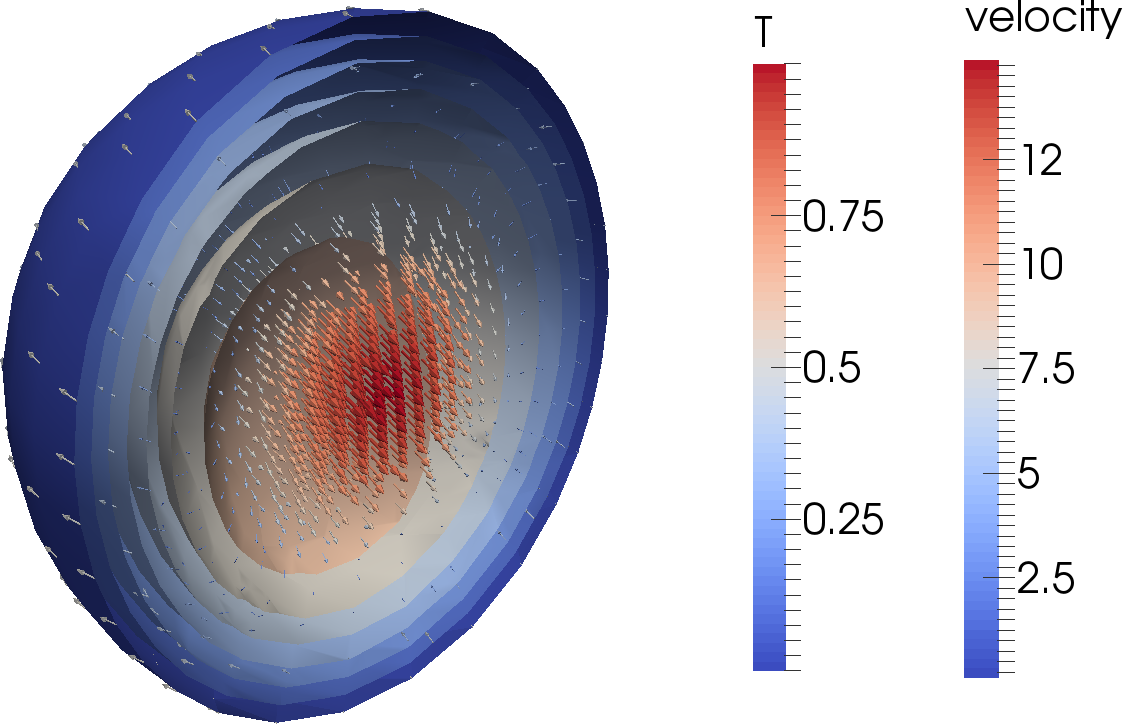
For low
(<29), the convective translation mode dominates, where material freezes at one side of the inner core and melts at
the other side, so that the velocity field is uniform, pointing from the freezing to the melting side. Otherwise, at high
(>29),
convection takes the usual form of thermal convection with shear free boundary and no phase change, that is the
one-cell axisymmetric mode at the onset, and chaotic plume convection for larger Rayleigh number. In this case,
melting and solidification at the ICB have only a small dynamic effect. At intermediate values of P, the first
unstable mode is a linear combination of the high-P convection mode and of the small-P translation
mode.
Changing the values of
and in
the input file allows switching between the different regimes. The Rayleigh number can be changed by adjusting the
magnitude of the gravity:
The phase change number is implemented as part of the material model, and as a function that can depend on the
spatial coordinates and/or on time:
Figure 58 shows examples of the three regimes with
(plume
convection),
(translation),
(no convection).
Mesh refinement. The temperature is set to 0 at the outer boundary and a large temperature gradient can develop at
the boundary layer, especially for the translation regime. The adaptive mesh refinement allows it to resolve this layer at
the inner core boundary. Another solution is to apply a specific initial refinement, based on the boundary layer thickness
scaling law ,
and to refine specifically the uppermost part of the inner core.
In order to have a mesh that is much finer at the outer boundary than in the center of the domain, this
expression for the mesh refinement subsection can be used in the input file:
Scaling laws. In addition, [DAC13] give scaling laws for the velocities in each regime derived from linear
stability analysis of perfect translation, and show how numerical results compare to them. In the regimes of low
,
translation will start at a critical ratio of Rayleigh number and phase change number
with steady-state translation velocities being zero below this threshold and tending to
going towards higher values of
. In the same way, translation
velocities will decrease from
with increasing , with translation
transitioning to plume convection at .
Both trends are shown in Figure 59 and can be compared to Figure 8 and 9 in [DAC13].
5.3.11 Melt migration in a 2D mantle convection model
This section was contributed by Juliane Dannberg and is based on a section in [DH16] by Juliane Dannberg and
Timo Heister.
The following cookbook will explain how to use ASPECT’s implementation of coupled magma/mantle dynamics
(see Section 2.13) to set up a model of mantle convection that also includes melting and freezing of mantle rock,
and the transport of melt according to the two-phase flow equations. The model setup is described in detail in
[DH16], which can be found here, and in the following we will go over a slightly simplified version in lower
resolution. We will start by looking at a global mantle convection without melt migration, and will then discuss how
the input file has to be modified in order to add melt transport. A movie that compares the evolution of the
temperature field and the amount of melt present in both models in higher resolution can be found
online.
The model setup is a 2D box with dimensions of
km, and
it is heated from the bottom and cooled from the top. A full description can be found in Section 4.7 “Influence of
melt migration on a global-scale convection model” in [DH16]. In the first model we will look at, melting and
freezing is only included passively: We use the melt fraction visualization postprocessor to compute how much
melt is present for a given temperature and pressure at every given point in time and space in our model, but the
presence of melt does not influence material properties like density or viscosity, and melt does not move
relative to the solid. This also means that because melt is not extracted, the bulk composition of the
material always stays the same, and melt only freezes again once advection or conduction causes the
temperature of the solid rock to be below the solidus. The following input file (which can be found in
cookbooks/global_no_melt.prm) contains a detailed description of the different options required to set up such a
model:
When we look at visualization output of this model, we can see that over time, first upwellings, and then
downwellings start to form. Both are more or less stable over time, and only change their positions slowly. As melt
does not move relative to the solid, broad stable zones of melting with melt fraction of 10% or more form in areas
where material is upwelling.
In the second model, melt is an active component of the model. Temperature, pressure and composition control
how much of the rock melts, and as soon as that happens, melt can migrate relative to the solid rock. As material
only melts partially, that means that the composition of the rock changes when it melts and melt is extracted, and
we track this change in composition using a compositional field with the name peridotite. Positive values mark
depletion (the composition of the residual host rock as more and more melt is extracted), and negative values mark
enrichment (the composition of generated melt, or regions where melt freezes again). Both the fraction of melt
(tracked by the compositional field with the name porosity) and the changes in composition influence the material
properties such as density and viscosity. Moreover, there are additional material properties that describe how
easily melt can move through the host rock, such as the permeability, or properties of the melt itself,
such as the fluid viscosity. The following input file (a complete version of which can be found in
cookbooks/global_melt.prm) details the changes we have to make from the first model to set up a model with
melt migration:
In the first few tens of millions of years, this models evolves similarly to the model without melt migration.
Upwellings rise in the same locations, and regions where material starts to melt are similar. However, once melt is
formed, the model evolutions start to deviate. In the model with melt migration, melt moves upwards from the
region where it is generated much faster than the flow of solid material, so that it reaches cold regions – where it
freezes again – in a shorter amount of time. Because of that, the overall amount of melt is smaller in this model at
any given point in time. In addition, enriched material, present in places where melt has crystallized, has a higher
density than average or depleted mantle material. This means that in regions above stable upwellings,
instabilities of dense, enriched material start to form, which leads to small-scale downwellings. Hence,
both areas where material is partially molten and the location of the upwellings themselves have a
much shorter wavelength and change much faster over time in comparison to the model without melt
migration.
Figure 60 shows the time evolution of both models. A more complete comparison of the two models can be
found in Section 4.7 “Influence of melt migration on a global-scale convection model” in [DH16].
5.3.12 Melt migration in a 2D mid-ocean ridge model
This section was contributed by Juliane Dannberg.
The following cookbook will explain how to set up a model of a mid-ocean ridge that uses ASPECT’s
implementation of coupled magma/mantle dynamics (see Section 2.13) and melting and freezing of mantle rock. In
particular, it will outline
- how to use operator splitting to accurately compute melting and freezing of melt,
- how to use traction boundary conditions to set up the flow field of a mid-ocean ridge,
- useful strategies for how to refine the mesh in models with melt migration.
How to set up a model with melt migration in general is explained in the previous cookbook 5.3.11.
As the flow at mid-ocean ridges can be assumed to be roughly symmetric with respect to the ridge
axis in the center, we only model one half of the ridge in a 2d Cartesian box with dimensions of
km.
Solid material is flowing in from the bottom with a prescribed temperature and melting due to decompression as is
rises. The model is cooled from the top so that melt freezes again as it approaches this boundary. In
addition, a fixed plate velocity away from the ridge axis is prescribed at the top boundary, inducing
corner flow. Material can flow out freely at the right model boundary. The model shows both how melt
is focused towards the ridge axis, and how melting and freezing induces chemical heterogeneity in
the mantle, generating the crust and lithosphere. A movie of the full model evolution can be found
online.
The input file.
One important problem in models with melting and freezing (and other reactions) is that these reactions can be
much faster than the time step of the model. For mid-ocean ridges, melt is generally assumed to be in equilibrium
with the solid, which means that the reaction is basically instantaneous. To model these type of processes,
ASPECT uses operator splitting (see also Section 5.4.15): Reactions are solved on a different time scale than
advection. For this model, this means that at the beginning of each time step, all melting reactions,
including their latent heat effects, are solved using several shorter sub-time steps. In the input file,
we have to choose both the size of these sub-time steps and the rate (or characteristic time scale) of
melting, and they have to be consistent in the sense that the operator splitting time step can not be
larger than the reaction time scale. The melting model we use here is the anhydrous mantle melting
model of [KSL03] for a peridotitic rock composition, as implemented in the “melt simple” material
model.
To make sure we reproduce the characteristic triangular melting region of a mid-ocean ridge, we have to set up
the boundary conditions in a way so that they will lead to corner flow. At the top boundary, we can simply prescribe
the half-spreading rate, and at the left boundary we can use a free-slip boundary, as material should not cross this
centerline. However, we do not know the inflow and outflow velocities at the bottom and right side of the model.
Instead, what we can do here is prescribing the lithostatic pressure as a boundary condition for the stress. We
accomplish this by using the “initial lithostatic pressure” model. This plugin will automatically compute a 1d
lithostatic pressure profile at a given point at the time of the model start and apply it as a boundary
traction.
Finally, we have to make sure that the resolution is high enough to model melt migration. This is particularly
important in regions where the porosity is low, but still high enough that the two-phase flow equations
are solved (instead of the Stokes system, which is solved if there is no melt present in a cell). At the
boundary between these regions, material properties like the compaction viscosity may jump, and
there may be strong gradients or jumps in some solution variables such as the melt velocity and the
compaction pressure. In addition, the characteristic length scale for melt transport, the compaction length
,
depends on the porosity:
|
| (54) |
While the melt viscosity
is usually assumed to be constant, and the shear and compaction viscosities
and
increase with
decreasing porosity ,
the permeability
or
dominates this relation, so that the compaction length becomes smaller for lower porosities. As the length scale of
melt migration is usually smaller than for mantle convection, we want to make sure that regions where melt is
present have a high resolution, and that this high resolution extends to all cells where the two-phase flow equations
are solved.
ASPECT also supports an alternative method to make sure that regions with melt are sufficiently well resolved,
relying directly on the compaction length, and we will discuss this method as a possible modification to this
cookbook at the end of this section.
The complete input file is located at cookbooks/mid_ocean_ridge.prm.
Model evolution.
When we look at the visualization output of this model (see also Figure 61), we can see how the hot material
flowing in from the bottom starts to melt as it reaches lower and lower pressures and crosses the solidus.
Simultaneously, melting makes the residual solid rock more depleted (as indicated by the positive values of the
compositional field called ‘peridotite’). Once material approaches the surface, it is cooled from the cold boundary
layer above, and melt starts to crystallize again, generating ‘enriched’ basaltic crust where is freezes (as indicated by
the negative values of the compositional field called ‘peridotite’). As the temperature gradients are much sharper
close to the surface, this transition from melt to solid rock is much sharper than in the melting region. Once
material crystallizes, it is transported away from the ridge axis due to the flow field induced by the prescribed plate
velocity at the top boundary. This way, over time, the classical triangular melting region develops at
the ridge axis, and the material transported away from the ridge shows two distinct layers: The top
km are enriched material, and form the basaltic crust (negative peridotite field), and the
km
below are depleted material, and form the lithosphere (positive peridotite field). A vertical profile at a distance of 80
km from the ridge axis showing this composition can be found in Figure 62.
Mesh refinement.
Another option for making sure that melt migration is resolved properly in the model is using a refinement
criterion that directly relates to the compaction length. This can be done in the mesh refinement section of the input
file:
This will lead to a higher resolution particularly in regions with low (but not zero) porosity, and can be useful to
resolve the strong gradients in the melt velocity and compaction pressure that are to be expected in
these places (see Figure 63). Of course it is also possible to combine both methods for refining the
mesh.
Extending the model.
There are a number of parameters that influence the amount of melting, how fast the melt moves, and
ultimately the distribution of crustal and lithospheric material. Some ideas for adapting the model setup:
- Changing the spreading rate: This can be done by choosing a different magnitude of the prescribed
velocity at the top boundary, and influences the size and shape of the triangular melting region. Faster
spreading allows hot material to move further away from the ridge axis, and hence facilitates a melting
region that extends further in horizontal direction.
- Changing the temperature profile: This can be done by choosing a different bottom boundary
temperature and influences the amount of melting, and hence the thickness of the crust. Higher
temperatures lead to more melt being generated.
- Changing the speed of melt migration: The velocity of the melt with respect to the solid velocity
is determined by the permeability and the melt viscosity (and the pressure gradients in the melt).
Increasing the permeability (by setting a different “Reference permeability” in the melt simple model)
can lead to higher melt velocities, melt reaching the depth of freezing faster, and hence lower overall
porosity values at steady state.
- Making the viscosity law more realistic: In this simple model, the viscosity only depends on the
amount of melt that is present and is otherwise constant. This could be the reason why melt can
not flow up all the way up at the ridge axis, but freezes before it reaches the surface. Introducing a
temperature-dependent rheology could improve this behavior (and in reality, plastic effects might also
play a role).