Benchmarks

5.4 Benchmarks

Benchmarks are used to verify that a solver solves the problem correctly, i.e., to verify correctness of a code.³⁵ Over the past decades, the geodynamics community has come up with a large number of benchmarks. Depending on the goals of their original inventors, they describe stationary problems in which only the solution of the flow problem is of interest (but the flow may be compressible or incompressible, with constant or variable viscosity, etc), or they may actually model time-dependent processes. Some of them have solutions that are analytically known and can be compared with, while for others, there are only sets of numbers that are approximately known. We have implemented a number of them in ASPECT to convince ourselves (and our users) that ASPECT indeed works as intended and advertised. Some of these benchmarks are discussed below. Numerical results for several of these benchmarks are also presented in [KHB12] in much more detail than shown here.

5.4.1 Running benchmarks that require code

Some of the benchmarks require plugins like custom material models, boundary conditions, or postprocessors. To not pollute ASPECT with all these purpose-built plugins, they are kept separate from the more generic plugins in the normal source tree. Instead, the benchmarks have all the necessary code in .cc files in the benchmark directories. Those are then compiled into a shared library that will be used by ASPECT if it is referenced in a .prm file. Let’s take the SolCx benchmark as an example (see Section 5.4.4). The directory contains:

solcx.cc – the code file containing a material model “SolCxMaterial” and a postprocessor “SolCxPostprocessor”,
solcx.prm – the parameter file referencing these plugins,
CMakeLists.txt – a cmake configuration that allows you to compile solcx.cc.

To run this benchmark you need to follow the general outline of steps discussed in Section 6.2. For the current case, this amounts to the following:

Move into the directory of that particular benchmark:
$ cd benchmarks/solcx
Set up the project:
$ cmake .

By default, cmake will look for the ASPECT binary and other information in a number of directories relative to the current one. If it is unable to pick up where ASPECT was built and installed, you can specify this directory explicitly this using -D Aspect_DIR= $<$ ... $>$ as an additional flag to cmake, where $<$ ... $>$ is the path to the build directory.
Build the library:
$ make

This will generate the file libsolcx.so.

Finally, you can run ASPECT with solcx.prm:

$ ../../aspect solcx.prm

where again you may have to use the appropriate path to get to the ASPECT executable. You will need to run ASPECT from the current directory because solcx.prm refers to the plugin as ./libsolcx.so, i.e., in the current directory.

5.4.2 Onset of convection benchmark

This section was contributed by Max Rudolph, based on a course assignment for “Geodynamic Modeling” at Portland State University.

Here we use ASPECT to numerically reproduce the results of a linear stability analysis for the onset of convection in a fluid layer heated from below. This exercise was assigned to students at Portland State University as a first step towards setting up a nominally Earth-like mantle convection model. Hence, representative length scales and transport properties for Earth are used. This cookbook consists of a jupyter notebook (benchmarks/onset-of-convection/onset-of-convection.ipynb) that is used to run ASPECT and analyze the results of several calculations. To use this code, you must compile ASPECT and give the path to the executable in the notebook as aspect_bin.

The linear stability analysis for the onset of convection appears in Turcotte and Schubert [TS14] (section 6.19). The linear stability analysis assumes the Boussinesq approximation and makes predictions for the growth rate (vertical velocity) of instabilities and the critical Rayleigh number $R a_{c r}$ above which convection will occur. $R a_{c r}$ depends only on the dimensionless wavelength of the perturbation, which is assumed to be equal to the width of the domain. The domain has height $b$ and width $λ$ and the perturbation is described by

\begin{array}{l} T^{'} (x, y) = T_{0}^{'} cos (\frac{2 π x}{λ}) sin (\frac{π y}{b}), \end{array}

where $T_{0}^{'}$ is the amplitude of the perturbation. Note that because we place the bottom boundary of the domain at $y = 0$ and the top at $y = b$ , the perturbation vanishes at the top and bottom boundaries. This departs slightly from the setup in [TS14], where the top and bottom boundaries of the domain are at $y = \pm b ∕ 2$ . The analytic expression for the critical Rayleigh number, $R a_{c r}$ is given in Turcotte and Schubert [TS14] equation (6.319):

\begin{array}{l} R a_{c r} = \frac{{(π^{2} + \frac{4 π^{2} b^{2}}{λ^{2}})}^{3}}{\frac{4 π^{2} b^{2}}{λ^{2}}} . \end{array}

The linear stability analysis also makes a prediction for the dimensionless growth rate of the instability $α^{'}$ (Turcotte and Schubert [TS14], equation (6.315)). The maximum vertical velocity is given by

\begin{array}{l} v_{y, m a x} = \frac{2 π}{λ} ϕ_{0}^{'} e^{α^{'} t}, \end{array}

where

\begin{array}{l} ϕ_{0}^{'} = - \frac{2 π}{λ} \frac{ρ_{0} g α T_{0}^{'}}{μ} {(\frac{4 π^{2}}{λ^{2}} + \frac{π^{2}}{b^{2}})}^{- 2}, \end{array}

and

\begin{array}{l} α^{'} = \frac{κ}{b^{2}} [\frac{ρ_{0} g α b^{3} Δ T}{μ κ} (\frac{\frac{4 π^{2} b^{2}}{λ^{2}}}{{(\frac{4 π^{2} b^{2}}{λ^{2}} + π^{2})}^{2}}) - (π^{2} + \frac{4 π^{2} b^{2}}{λ^{2}})] . \end{array}

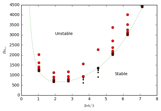
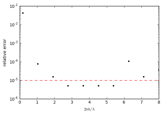
We use bisection to determine $R a_{c r}$ for specific choices of the domain geometry, keeping the depth $b$ constant and varying the domain width $λ$ . If the vertical velocity increases from the first to the second timetsp, the system is unstable to convection. Otherwise, it is stable and convection will not occur. Each calculation is terminated after the second timestep. Fig. 64 shows the numerically-determined threshold for the onset of convection, which can be compared directly with the theoretical prediction (green curve) and Fig. 6.39 of [TS14]. The relative error between the numerically-determined value of $R a_{c r}$ and the analytic solution are shown in the right panel of Fig. 64.

Figure 64: Left: Comparison of numerically-determined and theoretical values for

R a_{c r}

. Red circles indicate numerical simulations unstable to convection, black circles indicate simulations that are stable. The green dashed curve indicates the theoretical prediction. Right: Relative error in determination of

R a_{c r}

. The dashed red line indicates the error tolerance used in bisection procedure.

5.4.3 The van Keken thermochemical composition benchmark

This section is a co-production of Cedric Thieulot, Juliane Dannberg, Timo Heister and Wolfgang Bangerth with an extension to this benchmark provided by the Virginia Tech Department of Geosciences class “Geodynamics and ASPECT” co-taught by Scott King and D. Sarah Stamps.

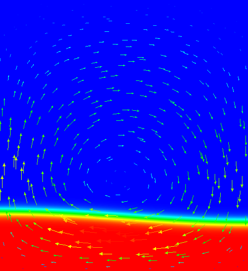
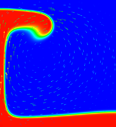
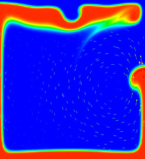
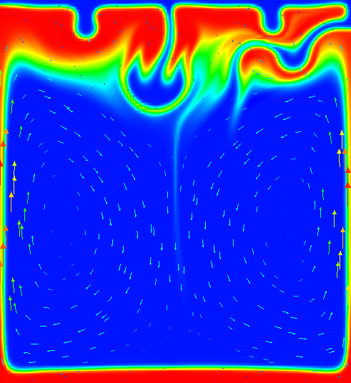
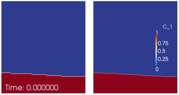
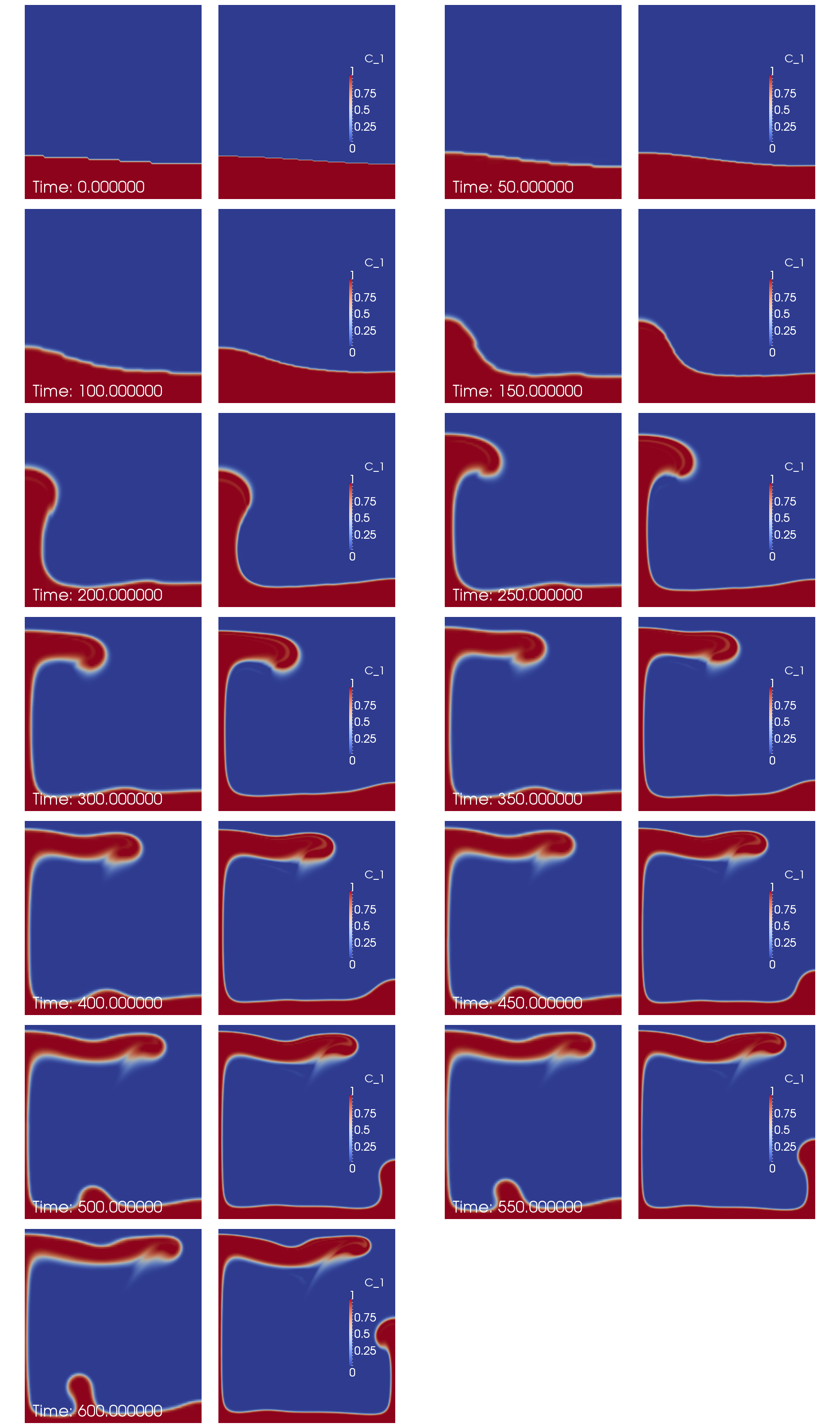
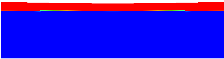
One of the most widely used benchmarks for mantle convection codes is the isoviscous Rayleigh-Taylor case (“case 1a”) published by van Keken et al. in [vKKS $^{+}$ 97]. The benchmark considers a 2d situation where a lighter fluid underlies a heavier one with a non-horizontal interface between the two of them. This unstable layering causes the lighter fluid to start rising at the point where the interface is highest. Fig. 65 shows a time series of images to illustrate this.

Figure 65: Van Keken benchmark (using a smoothed out interface, see the main text): Compositional field at times

t = 0, 300, 900, 1800

Although van Keken’s paper title suggests that the paper is really about thermochemical convection, the part we look here can equally be considered as thermal or chemical convection: all that is necessary is that we describe the fluid’s density somehow. We can do that by using an inhomogeneous initial temperature field, or an inhomogeneous initial composition field. We will use the input file in cookbooks/van-_keken-_discontinuous.prm as input, the central piece of which is as follows (go to the actual input file to see the remainder of the input parameters):

subsection ??
  set ?? = simple
  subsection ??
    set ??                     = 1e2
    set ?? = 0
    set ?? = -10
  end
end

subsection ??
  set ?? = function
  subsection ??
    set ??      = x,z
    set ??  = pi=3.14159
    set ?? = if( (z>0.2+0.02*cos(pi*x/0.9142)) , 0 , 1 )
  end
end

The first part of this selects the simple material model and sets the thermal expansion to zero (resulting in a density that does not depend on the temperature, making the temperature a passively advected field) and instead makes the density depend on the first compositional field. The second section prescribes that the first compositional field’s initial conditions are 0 above a line describes by a cosine and 1 below it. Because the dependence of the density on the compositional field is negative, this means that a lighter fluid underlies a heavier one.

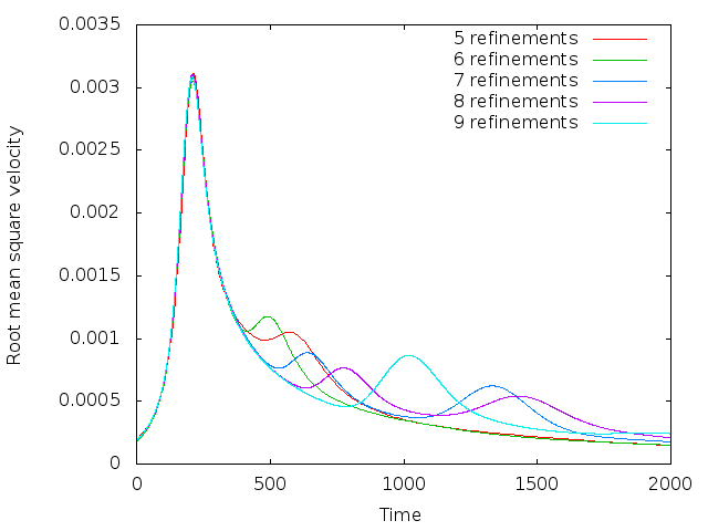
The dynamics of the resulting flow have already been shown in Fig. 65. The measure commonly considered in papers comparing different methods is the root mean square of the velocity, which we can get using the following block in the input file (the actual input file also enables other postprocessors):

subsection ??
set ?? = velocity statistics
end

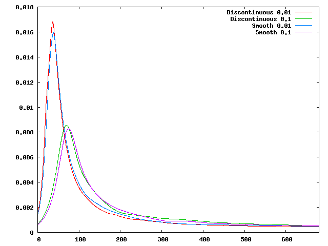
Using this, we can plot the evolution of the fluid’s average velocity over time, as shown in the left panel of Fig. 66. Looking at this graph, we find that both the timing and the height of the first peak is already well converged on a simple $32 \times 32$ mesh (5 global refinements) and is very consistent (to better than 1% accuracy) with the results in the van Keken paper.

Figure 66: Van Keken benchmark with discontinuous (left) and smoothed, continuous (right) initial conditions for the compositional field: Evolution of the root mean square velocity

{(\frac{1}{| Ω |} \int_{Ω} | u (x, t) |^{2} d x)}^{1 ∕ 2}

as a function of time for different numbers of global mesh refinements. 5 global refinements correspond to a

32 \times 32

mesh, 9 refinements to a

512 \times 512

mesh.

That said, it is startling that the second peak does not appear to converge despite the fact that the various codes compared in [vKKS $^{+}$ 97] show good agreement in this comparison. Tracking down the cause for this proved to be a lesson in benchmark design; in hindsight, it may also explain why van Keken et al. stated presciently in their abstract that “…good agreement is found for the initial rise of the unstable lower layer; however, the timing and location of the later smaller-scale instabilities may differ between methods.” To understand what is happening here, note that the first peak in these plots corresponds to the plume that rises along the left edge of the domain and whose evolution is primarily determined by the large-scale shape of the initial interface (i.e., the cosine used to describe the initial conditions in the input file). This is a first order deterministic effect, and is obviously resolved already on the coarsest mesh shown used. The second peak corresponds to the plume that rises along the right edge, and its origin along the interface is much harder to trace – its position and the timing when it starts to rise is certainly not obvious from the initial location of the interface. Now recall that we are using a finite element field using continuous shape functions for the composition that determines the density differences that drive the flow. But this interface is neither aligned with the mesh, nor can a discontinuous function be represented by continuous shape functions to begin with. In other words, we may input the initial conditions as a discontinuous functions of zero and one in the parameter file, but the initial conditions used in the program are in fact different: they are the interpolated values of this discontinuous function on a finite element mesh. This is shown in Fig. 67. It is obvious that these initial conditions agree on the large scale (the determinant of the first plume), but not in the steps that may (and do, in fact) determine when and where the second plume will rise. The evolution of the resulting compositional field is shown in Fig. 68 and it is obvious that the second, smaller plume starts to rise from a completely different location – no wonder the second peak in the root mean square velocity plot is in a different location and with different height!

Figure 67: Van Keken benchmark with discontinuous initial conditions for the compositional field: Initial compositional field interpolated onto a

32 \times 32

(left) and

64 \times 64

finite element mesh (right).

Figure 68: Van Keken benchmark with discontinuous initial conditions for the compositional field: Evolution of the compositional field over time on a

32 \times 32

(first and third column; left to right and top to bottom) and

64 \times 64

finite element mesh (second and fourth column).

The conclusion one can draw from this is that if the outcome of a computational experiment depends so critically on very small details like the steps of an initial condition, then it’s probably not a particularly good measure to look at in a benchmark. That said, the benchmark is what it is, and so we should try to come up with ways to look at the benchmark in a way that allows us to reproduce what van Keken et al. had agreed upon. To this end, note that the codes compared in that paper use all sorts of different methods, and one can certainly agree on the fact that these methods are not identical on small length scales. One approach to make the setup more mesh-independent is to replace the original discontinuous initial condition with a smoothed out version; of course, we can still not represent it exactly on any given mesh, but we can at least get closer to it than for discontinuous variables. 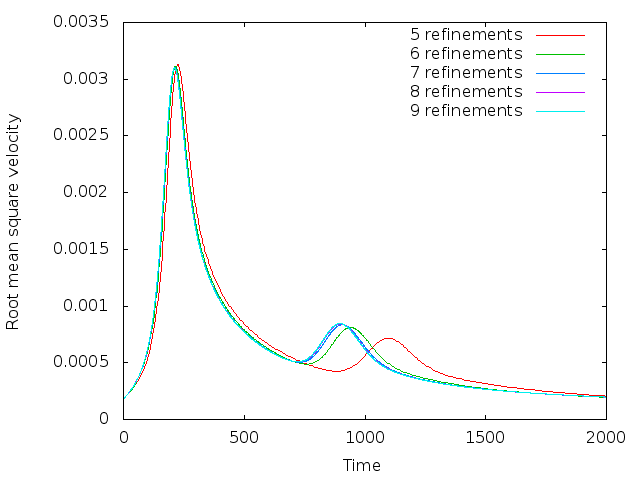Consequently, let us use the following initial conditions instead (see also the file cookbooks/van-_keken-_smooth.prm):

subsection ??
  set ?? = function
  subsection ??
    set ??      = x,z
    set ??  = pi=3.14159
    set ?? = 0.5*(1+tanh((0.2+0.02*cos(pi*x/0.9142)-z)/0.02))
  end
end

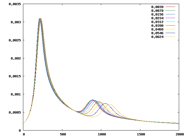
This replaces the discontinuous initial conditions with a smoothed out version with a half width of around 0.01. Using this, the root mean square plot now looks as shown in the right panel of Fig. 66. Here, the second peak also converges quickly, as hoped for.

The exact location and height of the two peaks is in good agreement with those given in the paper by van Keken et al., but not exactly where desired (the error is within a couple of per cent for the first peak, and probably better for the second, for both the timing and height of the peaks). This has to do with the fact that they depend on the exact size of the smoothing parameter (the division by 0.02 in the formula for the smoothed initial condition). However, for more exact results, one can choose this half width parameter proportional to the mesh size and thereby get more accurate results. The point of the section was to demonstrate the reason for the lack of convergence.

In this section we extend the van Keken cookbook following up the work previously completed by Cedric Thieulot, Juliane Dannberg, Timo Heister and Wolfgang Bangerth. This section contributed by Grant Euen, Tahiry Rajaonarison, and Shangxin Liu as part of the Geodynamics and ASPECT class at Virginia Tech.

As already mentioned above, using a half width parameter proportional to the mesh size allows for more accurate results. We test the effect of the half width size of the smoothed discontinuity by changing the division by 0.02, the smoothing parameter, in the formula for the smoothed initial conditions into values proportional to the mesh size. We use 7 global refinements because the root mean square velocity converges at greater resolution while keeping average runtime around 5 to 25 minutes. These runtimes were produced by the BlueRidge cluster of the Advanced Research Computing (ARC) program at Virginia Tech. BlueRidge is a 408-node Cray CS-300 cluster; each node outfitted with two octa-core Intel Sandy Bridge CPUs and 64 GB of memory. A chart of average runtimes for 5 through 10 global refinements on one node can be seen in Table 5. For 7 global refinements (128 $\times$ 128 mesh size), the size of the mesh is 0.0078 corresponding to a half width parameter of 0.0039. The smooth model allows for much better convergence of the secondary plumes, although they are still more scattered than the primary plumes.


Global	Number of Processors
Refinements	4	8	12	16

5	28.1 seconds	19.8 seconds	19.6 seconds	17.1 seconds
6	3.07 minutes	1.95 minutes	1.49 minutes	1.21 minutes
7	23.33 minutes	13.92 minutes	9.87 minutes	7.33 minutes
8	3.08 hours	1.83 hours	1.30 hours	56.33 minutes
9	1.03 days	15.39 hours	10.44 hours	7.53 hours
10	More than 6 days	More than 6 days	3.39 days	2.56 days

Table 5: Average runtimes for the van Keken Benchmark with smoothed initial conditions. These times are for the entire computation, a final time step number of 2000. All of these tests were run using ASPECT version 1.3 in release mode, and used different numbers of processors on one node on the BlueRidge cluster of ARC at Virginia Tech.

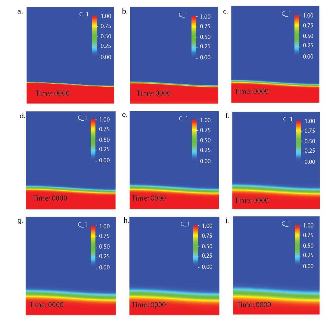
This convergence is due to changing the smoothing parameter, which controls how much of the problem is smoothed over. As the parameter is increased, the smoothed boundary grows and vice versa. As the smoothed boundary shrinks it becomes sharper until the original discontinuous behavior is revealed. As it grows, the two layers eventually become one large, transitioning layer rather than two distinct layers separated by a boundary. These effects can be seen in Fig. 69. The overall effect is that the secondary rise is at different times based on these conditions. In general, as the smoothing parameter is decreased, the smoothed boundary shrinks and the plumes rise more quickly. As it is increased, the boundary grows and the plumes rise more slowly. This trend can be used to force a more accurate convergence from the secondary plumes.

Figure 69: Van Keken Benchmark using smoothed out interface at 7 global refinements: compositional field at time

t = 0

using smoothing parameter size: a) 0.0039, b) 0.0078, c) 0.0156, d) 0.0234, e) 0.0312, f) 0.0390, g) 0.0468, h) 0.0546, i) 0.0624.

The evolution in time of the resulting compositional fields (Fig. 70) shows that the first peak converges as the smoothed interface decreases. There is a good agreement for the first peak for all smoothing parameters. As the width of the discontinuity increases, the second peak rises both later and more slowly.

Figure 70: Van Keken benchmark with smoothed initial conditions for the compositional field using 7 global refinements for different smoothing parameters. Number of the time step is shown on the

x

-axis, while root mean square velocity is shown on the

y

-axis.

Now let us further add a two-layer viscosity model to the domain. This is done to recreate the two nonisoviscous Rayleigh-Taylor instability cases (“cases 1b and 1c”) published in van Keken et al. in [vKKS $^{+}$ 97]. Let’s assume the viscosity value of the upper heavier layer is $η_{t}$ and the viscosity value of the lower lighter layer is $η_{b}$ . Based on the initial constant viscosity value 1 $\times 1 0^{2}$ Pa s, we set the viscosity proportion $\frac{η_{t}}{η_{b}} = 0.1, 0.01$ , meaning the viscosity of the upper, heavier layer is still 1 $\times 1 0^{2}$ Pa s, but the viscosity of the lower, lighter layer is now either 10 or 1 Pa s, respectively. 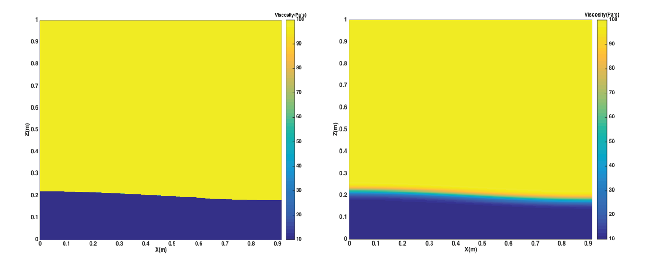The viscosity profiles of the discontinuous and smooth models are shown in Fig. 71.

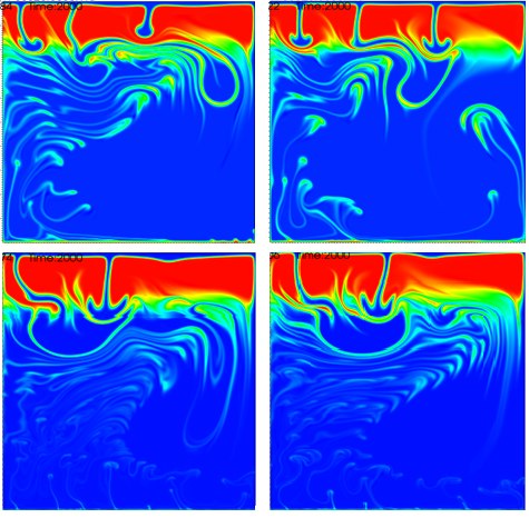
Figure 71: Van Keken benchmark using layers of different viscosities. The left image is the discontinuous case, while right is the smooth. Both are shown at t=0.

For both benchmark cases, discontinuous and smooth, and both viscosity proportions, 0.1 and 0.01, the results are shown at the end time step number, 2000, in Fig. 72. This was generated using the original input parameter file, running the cases with 8 global refinement steps, and also adding the two-layer viscosity model.

Figure 72: Van Keken benchmark two-layer viscosity model at final time step number, 2000. These images show layers of different compositions and viscosities. Discontinuous cases are the left images, smooth cases are the right. The upper images are

\frac{η_{t}}{η_{b}} = 0.1

, and the lower are

\frac{η_{t}}{η_{b}} = 0.01

Compared to the results of the constant viscosity throughout the domain, the plumes rise faster when adding the two-layer viscosity model. Also, the larger the viscosity difference is, the earlier the plumes appear and the faster their ascent. To further reveal the effect of the two-layer viscosity model, we also plot the evolution of the fluids’ average velocity over time, as shown in Fig. 73.

Figure 73: Van Keken benchmark: Evolution of the root mean square velocity as a function of time for different viscosity contrast proportions (0.1/0.01) for both discontinuous and smooth models.

We can observe that when the two-layer viscosity model is added, there is only one apparent peak for each case. The first peaks of the 0.01 viscosity contrast tests appear earlier and are larger in magnitude than those of 0.1 viscosity contrast tests. There are no secondary plumes and the whole system tends to reach stability after around 500 time steps.

5.4.4 The SolCx Stokes benchmark

The SolCx benchmark is intended to test the accuracy of the solution to a problem that has a large jump in the viscosity along a line through the domain. Such situations are common in geophysics: for example, the viscosity in a cold, subducting slab is much larger than in the surrounding, relatively hot mantle material.

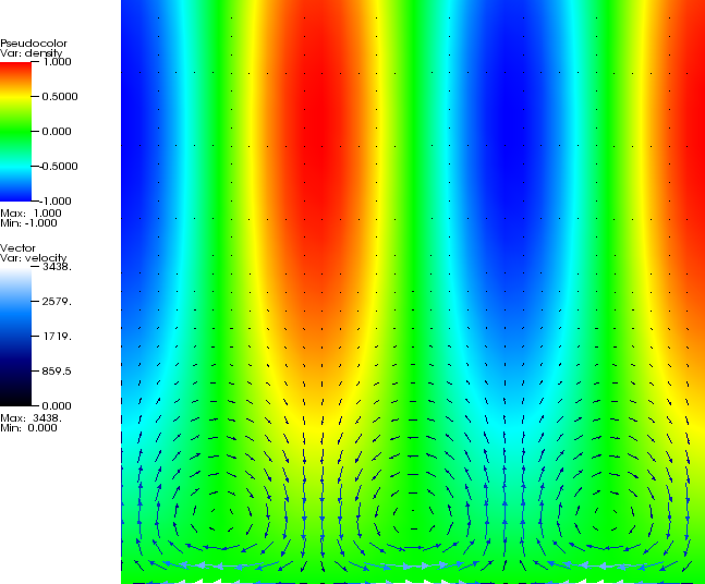
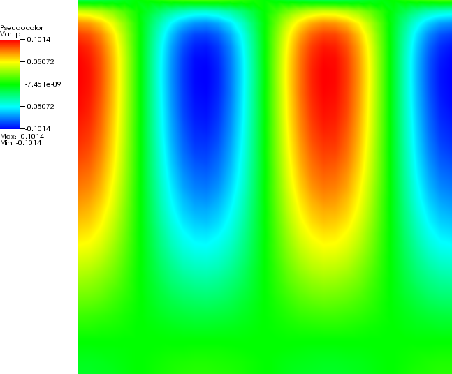
The SolCx benchmark computes the Stokes flow field of a fluid driven by spatial density variations, subject to a spatially variable viscosity. Specifically, the domain is $Ω = {[0, 1]}^{2}$ , gravity is $g = {(0, - 1)}^{T}$ and the density is given by $ρ (x) = sin (π x_{1}) cos (π x_{2})$ ; this can be considered a density perturbation to a constant background density. The viscosity is

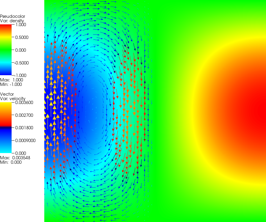
\begin{array}{l} η (x) = \{\begin{matrix} 1 & for x_{1} \leq 0.5, \\ 1 0^{6} & for x_{1} > 0.5 . \end{matrix} \end{array}

This strongly discontinuous viscosity field yields an almost stagnant flow in the right half of the domain and consequently a singularity in the pressure along the interface. Boundary conditions are free slip on all of $\partial Ω$ . The temperature plays no role in this benchmark. The prescribed density field and the resulting velocity field are shown in Fig. 74.

The SolCx benchmark was previously used in [DMGT11, Section 4.1.1] (references to earlier uses of the benchmark are available there) and its analytic solution is given in [Zho96]. ASPECT contains an implementation of this analytic solution taken from the Underworld package (see [MQL $^{+}$ 07] and http://www.underworldproject.org/, and correcting for the mismatch in sign between the implementation and the description in [DMGT11]).

Figure 74: SolCx Stokes benchmark. Left: The density perturbation field and overlaid to it some velocity vectors. The viscosity is very large in the right hand, leading to a stagnant flow in this region. Right: The pressure on a relatively coarse mesh, showing the internal layer along the line where the viscosity jumps.

To run this benchmark, the following input file will do (see the files in benchmarks/solcx/ to rerun the benchmark):

set ??            = ./libsolcx.so

############### Global parameters

set ??                              = 2

set ??                             = 0
set ??                               = 0

set ??                       = output

set ??                 = volume

############### Parameters describing the model

subsection ??
  set ?? = box

  subsection ??
    set ?? = 1
    set ?? = 1
  end
end

subsection ??
  set ?? = left, right, bottom, top
end

subsection ??
  set ?? = SolCxMaterial

  subsection ??
    set ?? = 1e6
  end
end

subsection ??
  set ?? = vertical
end

############### Parameters describing the temperature field

subsection ??
  set ?? = box
end

subsection ??
  set ?? = perturbed box
end

############### Parameters describing the discretization

subsection ??
  set ??       = 2
  set ?? = false
end

subsection ??
  set ??              = 0
  set ??                = 4
end

############### Parameters describing what to do with the solution

subsection ??
  set ?? = SolCxPostprocessor, visualization
end

Since this is the first cookbook in the benchmarking section, let us go through the different parts of this file in more detail:

The material model and the postprocessor
The first part consists of parameter setting for overall parameters. Specifically, we set the dimension in which this benchmark runs to two and choose an output directory. Since we are not interested in a time dependent solution, we set the end time equal to the start time, which results in only a single time step being computed.
The last parameter of this section, Pressure normalization, is set in such a way that the pressure is chosen so that its domain average is zero, rather than the pressure along the surface, see Section 2.5.
The next part of the input file describes the setup of the benchmark. Specifically, we have to say how the geometry should look like (a box of size $1 \times 1$ ) and what the velocity boundary conditions shall be (tangential flow all around – the box geometry defines four boundary indicators for the left, right, bottom and top boundaries, see also Section ??). This is followed by subsections choosing the material model (where we choose a particular model implemented in ASPECT that describes the spatially variable density and viscosity fields, along with the size of the viscosity jump) and finally the chosen gravity model (a gravity field that is the constant vector ${(0, - 1)}^{T}$ , see Section ??).
The part that follows this describes the boundary and initial values for the temperature. While we are not interested in the evolution of the temperature field in this benchmark, we nevertheless need to set something. The values given here are the minimal set of inputs.
The second-to-last part sets discretization parameters. Specifically, it determines what kind of Stokes element to choose (see Section ?? and the extensive discussion in [KHB12]). We do not adaptively refine the mesh but only do four global refinement steps at the very beginning. This is obviously a parameter worth playing with.
The final section on postprocessors determines what to do with the solution once computed. Here, we do two things: we ask ASPECT to compute the error in the solution using the setup described in the Duretz et al. paper [DMGT11], and we request that output files for later visualization are generated and placed in the output directory. The functions that compute the error automatically query which kind of material model had been chosen, i.e., they can know whether we are solving the SolCx benchmark or one of the other benchmarks discussed in the following subsections.

Upon running ASPECT with this input file, you will get output of the following kind (obviously with different timings, and details of the output may also change as development of the code continues):

aspect/cookbooks> ../aspect solcx.prm
Number of active cells: 256 (on 5 levels)
Number of degrees of freedom: 3,556 (2,178+289+1,089)

*** Timestep 0:  t=0 years
   Solving temperature system... 0 iterations.
   Rebuilding Stokes preconditioner...
   Solving Stokes system... 30+3 iterations.

   Postprocessing:
     Errors u_L1, p_L1, u_L2, p_L2: 1.125997e-06, 2.994143e-03, 1.670009e-06, 9.778441e-03
     Writing graphical output:      output/solution/solution-00000

+---------------------------------------------+------------+------------+
| Total wallclock time elapsed since start    |      1.51s |            |
|                                             |            |            |
| Section                         | no. calls |  wall time | % of total |
+---------------------------------+-----------+------------+------------+
| Assemble Stokes system          |         1 |     0.114s |       7.6% |
| Assemble temperature system     |         1 |     0.284s |        19% |
| Build Stokes preconditioner     |         1 |    0.0935s |       6.2% |
| Build temperature preconditioner|         1 |    0.0043s |      0.29% |
| Solve Stokes system             |         1 |    0.0717s |       4.8% |
| Solve temperature system        |         1 |  0.000753s |      0.05% |
| Postprocessing                  |         1 |     0.627s |        42% |
| Setup dof systems               |         1 |      0.19s |        13% |
+---------------------------------+-----------+------------+------------+

One can then visualize the solution in a number of different ways (see Section 4.4), yielding pictures like those shown in Fig. 74. One can also analyze the error as shown in various different ways, for example as a function of the mesh refinement level, the element chosen, etc.; we have done so extensively in [KHB12].

5.4.5 The SolKz Stokes benchmark

The SolKz benchmark is another variation on the same theme as the SolCx benchmark above: it solves a Stokes problem with a spatially variable viscosity but this time the viscosity is not a discontinuous function but grows exponentially with the vertical coordinate so that it’s overall variation is again $1 0^{6}$ . The forcing is again chosen by imposing a spatially variable density variation. For details, refer again to [DMGT11].

The following input file, only a small variation of the one in the previous section, solves the benchmark (see benchmarks/solkz/):

# A description of the SolKZ benchmark for which a known solution
# is available. See the manual for more information.

set ??            = ./libsolkz.so

############### Global parameters

set ??                              = 2

set ??                             = 0
set ??                               = 0

set ??                       = output

set ??                 = volume

############### Parameters describing the model

subsection ??
  set ?? = box

  subsection ??
    set ?? = 1
    set ?? = 1
  end
end

subsection ??
  set ?? = left, right, bottom, top
end

subsection ??
  set ?? = SolKzMaterial
end

subsection ??
  set ?? = vertical
end

############### Parameters describing the temperature field

subsection ??
  set ?? = box
end

subsection ??
  set ?? = perturbed box
end

############### Parameters describing the discretization

subsection ??
  set ??       = 2
  set ?? = false
end

subsection ??
  set ??              = 0
  set ??                = 4
end

############### Parameters describing what to do with the solution

subsection ??
  set ?? = SolKzPostprocessor, visualization
end

The output when running ASPECT on this parameter file looks similar to the one shown for the SolCx case. The solution when computed with one more level of global refinement is visualized in Fig. 75.

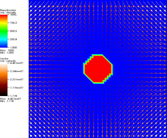
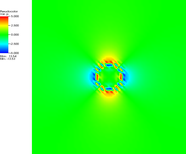
Figure 75: SolKz Stokes benchmark. Left: The density perturbation field and overlaid to it some velocity vectors. The viscosity grows exponentially in the vertical direction, leading to small velocities at the top despite the large density variations. Right: The pressure.

5.4.6 The “inclusion” Stokes benchmark

The “inclusion” benchmark again solves a problem with a discontinuous viscosity, but this time the viscosity is chosen in such a way that the discontinuity is along a circle. This ensures that, unlike in the SolCx benchmark discussed above, the discontinuity in the viscosity never aligns to cell boundaries, leading to much larger difficulties in obtaining an accurate representation of the pressure. Specifically, the almost discontinuous pressure along this interface leads to oscillations in the numerical solution. This can be seen in the visualizations shown in Fig. 76. As before, for details we refer to [DMGT11]. The analytic solution against which we compare is given in [SP03]. An extensive discussion of convergence properties is given in [KHB12].

Figure 76: Inclusion Stokes benchmark. Left: The viscosity field when interpolated onto the mesh (internally, the “exact” viscosity field – large inside a circle, small outside – is used), and overlaid to it some velocity vectors. Right: The pressure with its oscillations along the interface. The oscillations become more localized as the mesh is refined.

The benchmark can be run using the parameter files in benchmarks/inclusion/. The material model, boundary condition, and postprocessor are defined in benchmarks/inclusion/inclusion.cc. Consequently, this code needs to be compiled into a shared lib before you can run the tests.

Link to a general section on how you can compile libs for the benchmarks.

Revisit this once we have the machinery in place to choose nonzero boundary conditions in a more elegant way.

The following prm file isn’t annotated yet. How to annotate if we have a .lib?

############### Global parameters

set ??            = ./libinclusion.so

set ??                              = 2

set ??                             = 0
set ??                               = 0

set ??                       = output

set ??                 = volume

############### Parameters describing the model

subsection ??
  set ?? = box

  subsection ??
    set ?? = 2
    set ?? = 2
  end
end

subsection ??
  set ?? = left  : InclusionBoundary, \
                                                right : InclusionBoundary, \
                                                bottom: InclusionBoundary, \
                                                top   : InclusionBoundary
end

subsection ??
  set ?? = InclusionMaterial

  subsection ??
    set ?? = 1e3
  end
end

subsection ??
  set ?? = vertical
end

############### Parameters describing the temperature field

subsection ??
  set ?? = box
end

subsection ??
  set ?? = perturbed box
end

############### Parameters describing the discretization

subsection ??
  set ??       = 2
  set ?? = false
end

subsection ??
  set ??              = 0
  set ??                = 6
end

############### Parameters describing what to do with the solution

subsection ??
  set ?? = InclusionPostprocessor, visualization
end

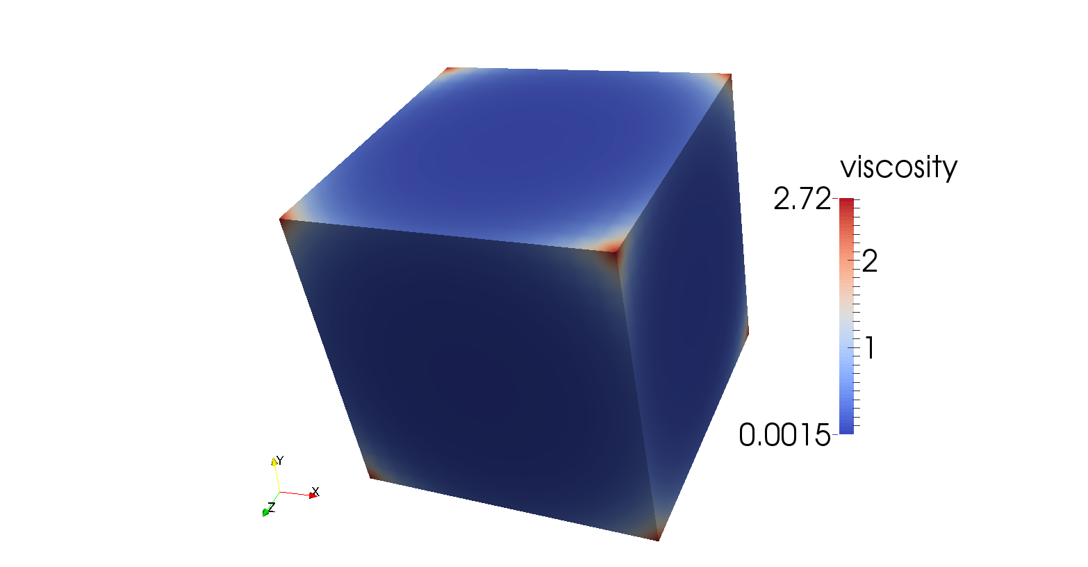
5.4.7 The Burstedde variable viscosity benchmark

This section was contributed by Iris van Zelst.

This benchmark is intended to test solvers for variable viscosity Stokes problems. It begins with postulating a smooth exact polynomial solution to the Stokes equation for a unit cube, first proposed by [DB14] and also described by [BSA $^{+}$ 13]:

\begin{align} u & = (\begin{matrix} x + x^{2} + x y + x^{3} y \\ y + x y + y^{2} + x^{2} y^{2} \\ - 2 z - 3 x z - 3 y z - 5 x^{2} y z \end{matrix}) & (55) \\ p & = x y z + x^{3} y^{3} z - \frac{5}{32} . & (56) \end{align}

It is then trivial to verify that the velocity field is divergence-free. The constant $- \frac{5}{32}$ has been added to the expression of $p$ to ensure that the volume pressure normalization of ASPECT can be used in this benchmark (in other words, to ensure that the exact pressure has mean value zero and, consequently, can easily be compared with the numerically computed pressure). Following [BSA $^{+}$ 13], the viscosity $μ$ is given by the smoothly varying function

μ = exp \{1 - β [x (1 - x) + y (1 - y) + z (1 - z)]\} .

(57)

The maximum of this function is $μ = e$ , for example at $(x, y, z) = (0, 0, 0)$ , and the minimum of this function is $μ = exp (1 - \frac{3 β}{4})$ at $(x, y, z) = (0.5, 0.5, 0.5)$ . The viscosity ratio $μ^{*}$ is then given by

μ^{*} = \frac{exp (1 - \frac{3 β}{4})}{exp (1)} = exp (\frac{- 3 β}{4}) .

(58)

Hence, by varying $β$ between 1 and 20, a difference of up to 7 orders of magnitude viscosity is obtained. $β$ will be one of the parameters that can be selected in the input file that accompanies this benchmark.

The corresponding body force of the Stokes equation can then be computed by inserting this solution into the momentum equation,

\nabla p - \nabla \cdot (2 μ ϵ (u)) = ρ g .

(59)

Using equations (55), (56) and (57) in the momentum equation (59), the following expression for the body force $ρ g$ can be found:

\begin{matrix} ρ g = (\begin{matrix} y z + 3 x^{2} y^{3} z \\ x z + 3 x^{3} y^{2} z \\ x y + x^{3} y^{3} \end{matrix}) - μ (\begin{matrix} 2 + 6 x y \\ 2 + 2 x^{2} + 2 y^{2} \\ - 10 y z \end{matrix}) \\ + (1 - 2 x) β μ (\begin{matrix} 2 + 4 x + 2 y + 6 x^{2} y \\ x + y + 2 x y^{2} + x^{3} \\ - 3 z - 10 x y z \end{matrix}) + (1 - 2 y) β μ (\begin{matrix} x + y + 2 x y^{2} + x^{3} \\ 2 + 2 x + 4 y + 4 x^{2} y \\ - 3 z - 5 x^{2} z \end{matrix}) \\ + (1 - 2 z) β μ (\begin{matrix} - 3 z - 10 x y z \\ - 3 z - 5 x^{2} z \\ - 4 - 6 x - 6 y - 10 x^{2} y \end{matrix}) & (60) \end{matrix}

Assuming $ρ = 1$ , the above expression translates into an expression for the gravity vector $g$ . This expression for the gravity (even though it is completely unphysical), has consequently been incorporated into the BursteddeGravity gravity model that is described in the benchmarks/burstedde/burstedde.cc file that accompanies this benchmark.

We will use the input file benchmarks/burstedde/burstedde.prm as input, which is very similar to the input file benchmarks/inclusion/adaptive.prm discussed above in Section 5.4.6. The major changes for the 3D polynomial Stokes benchmark are listed below:

subsection ??
  subsection ??
    set ??                = 1e-12
  end
end

# Boundary conditions
subsection ??
  set ?? = left  : BursteddeBoundary, \
                                                right : BursteddeBoundary, \
                                                front : BursteddeBoundary, \
                                                back  : BursteddeBoundary, \
                                                bottom: BursteddeBoundary, \
                                                top   : BursteddeBoundary
end

subsection ??
  set ?? = BursteddeMaterial
end

subsection ??
  set ?? = BursteddeGravity
end

subsection ??
   # Viscosity parameter is beta
   set ??             = 20
end

subsection ??
  set ?? = visualization, velocity statistics, BursteddePostprocessor
end

The boundary conditions that are used are simply the velocities from equation (55) prescribed on each boundary. The viscosity parameter in the input file is $β$ . Furthermore, in order to compute the velocity and pressure $L_{1}$ and $L_{2}$ norm, the postprocessor BursteddePostprocessor is used. Please note that the linear solver tolerance is set to a very small value (deviating from the default value), in order to ensure that the solver can solve the system accurately enough to make sure that the iteration error is smaller than the discretization error.

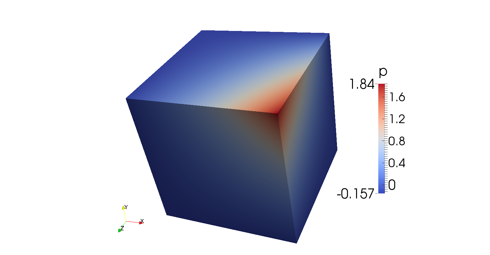
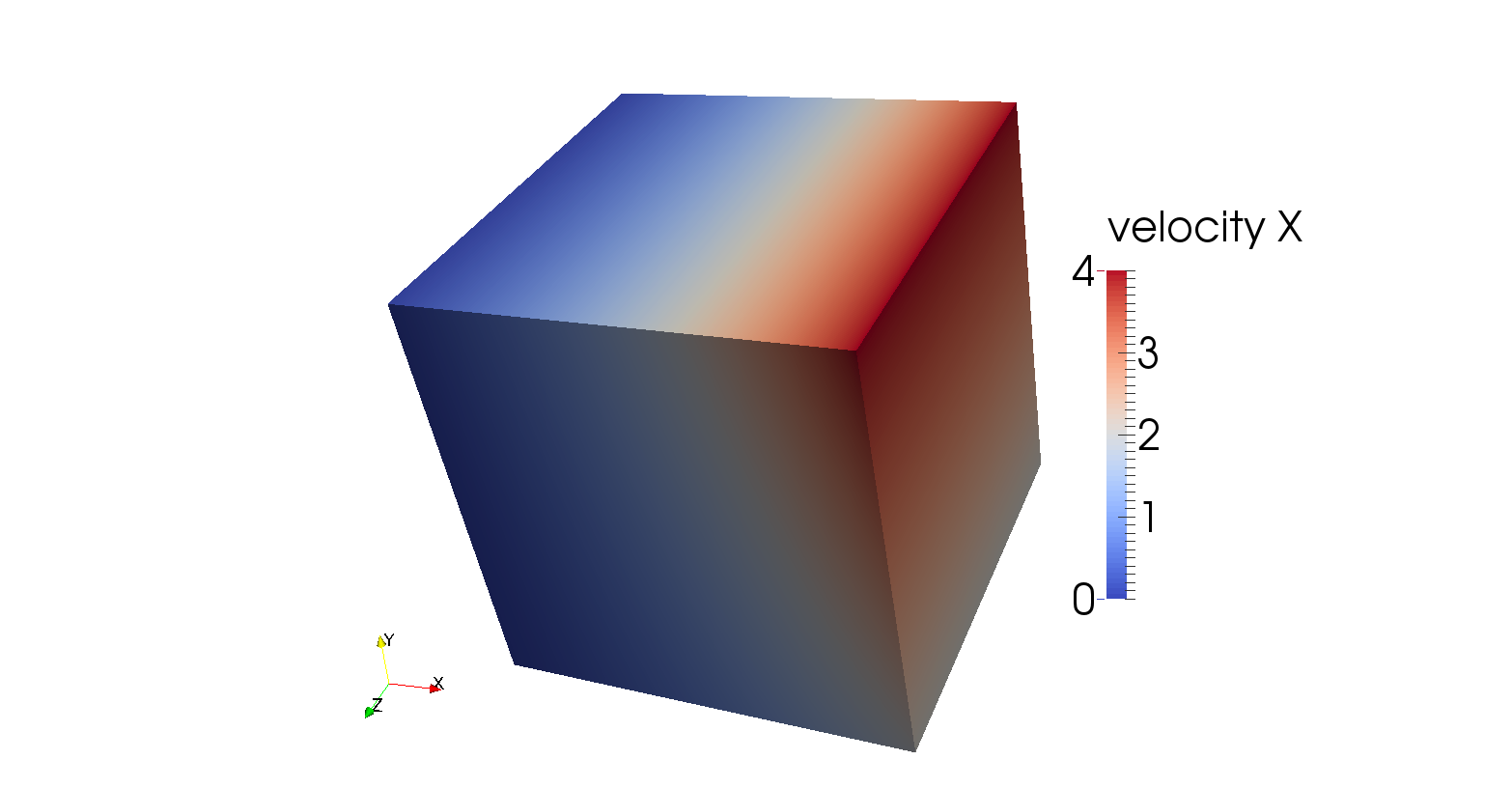
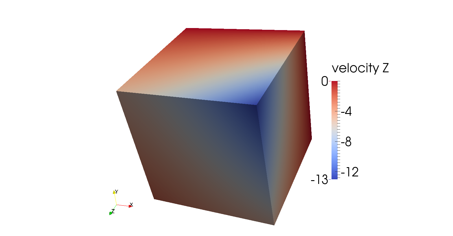
Expected analytical solutions at two locations are summarised in Table 6 and can be deduced from equations (55) and (56). Figure 77 shows that the analytical solution is indeed retrieved by the model.

Table 6: Analytical solutions

Quantity	$r = (0, 0, 0)$	$r = (1, 1, 1)$

$p$	$- 0.15625$	$1.84375$
$u$	$(0, 0, 0)$	$(4, 4, - 13)$
$\| u \|$	$0$	$14.177$

(a)

(b)

(c)

(d)

Figure 77: Burstedde benchmark: Results for the 3D polynomial Stokes benchmark, obtained with a resolution of

16 \times 16

elements, with

β = 10

The convergence of the numerical error of this benchmark has been analysed by playing with the mesh refinement level in the input file, and results can be found in Figure 78. The velocity shows cubic error convergence, while the pressure shows quadratic convergence in the $L_{1}$ and $L_{2}$ norms, as one would hope for using $Q_{2}$ elements for the velocity and $Q_{1}$ elements for the pressure.

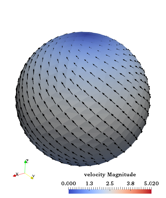
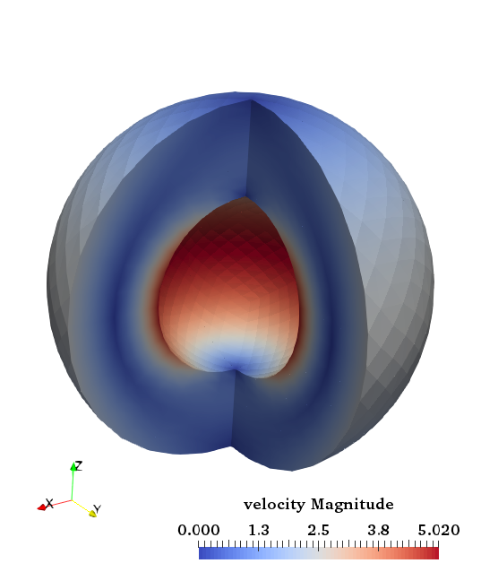
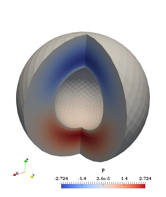
Figure 78: Burstedde benchmark: Error convergence for the 3D polynomial Stokes benchmark.

5.4.8 The hollow sphere benchmark

This benchmark is based on Thieulot [In prep.] in which an analytical solution to the isoviscous incompressible Stokes equations is derived in a spherical shell geometry. The velocity and pressure fields are as follows:

\begin{array}{rcl} v_{r} (r, θ) & = & g (r) cos θ, & (61) \\ v_{θ} (r, θ) & = & f (r) sin θ, & (62) \\ v_{ϕ} (r, θ) & = & f (r) sin θ, & (63) \\ p (r, θ) & = & h (r) cos θ, & (64) \end{array}

where

\begin{array}{rcl} f (r) & = & \frac{α}{r^{2}} + β r, & (65) \\ g (r) & = & - \frac{2}{r^{2}} (α ln r + \frac{β}{3} r^{3} + γ), & (66) \\ h (r) & = & \frac{2 μ_{0}}{r} g (r), & (67) \end{array}

with

\begin{array}{rcl} α & = & - γ \frac{R_{2}^{3} - R_{1}^{3}}{R_{2}^{3} ln R_{1} - R_{1}^{3} ln R_{2}}, & (68) \\ β & = & - 3 γ \frac{ln R_{2} - ln R_{1}}{R_{1}^{3} ln R_{2} - R_{2}^{3} ln R_{1}} . & (69) \end{array}

These two parameters are chosen so that $v_{r} (R_{1}) = v_{r} (R_{2}) = 0$ , i.e. the velocity is tangential to both inner and outer surfaces. The gravity vector is radial and of unit length, while the density is given by:

ρ (r, θ) = (\frac{α}{r^{4}} (8 ln r - 6) + \frac{8 β}{3 r} + 8 \frac{γ}{r^{4}}) cos θ .

(70)

We set $R_{1} = 0.5$ , $R_{2} = 1$ and $γ = - 1$ . The pressure is zero on both surfaces so that the surface pressure normalization is used. The boundary conditions that are used are simply the analytical velocity prescribed on both boundaries. The velocity and pressure fields are shown in Fig. 79.

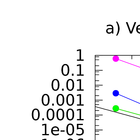
Fig. 80 shows the velocity and pressure errors in the $L_{2}$ -norm as a function of the mesh size $h$ (taken in this case as the radial extent of the elements). As expected we recover a third-order convergence rate for the velocity and a second-order convergence rate for the pressure.

Figure 79: Velocity and pressure fields for the hollow sphere benchmark.

Figure 80: Velocity and pressure errors in the

L_{2}

-norm as a function of the mesh size.

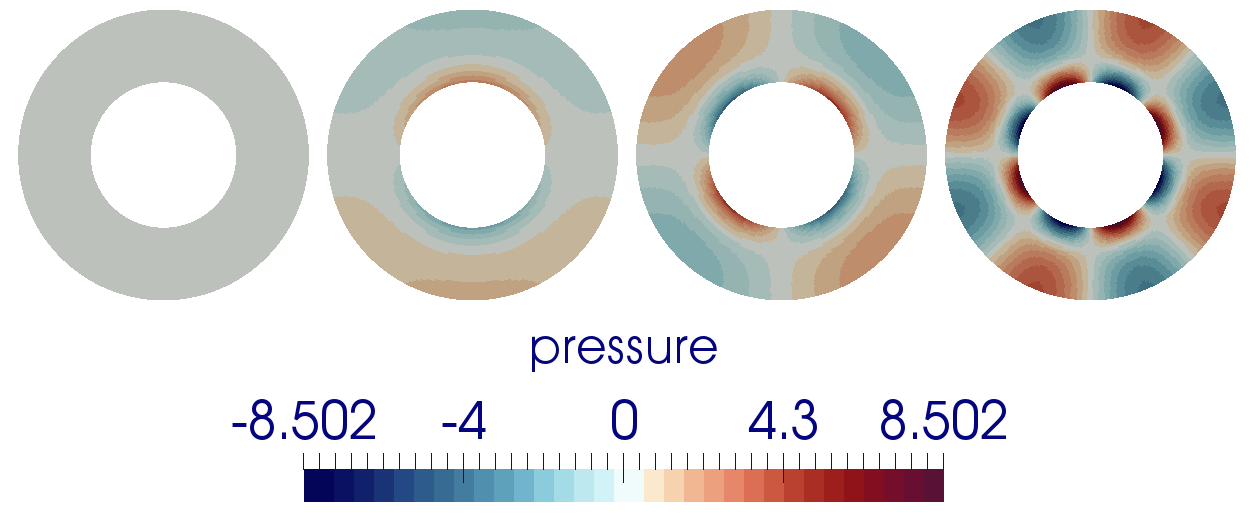
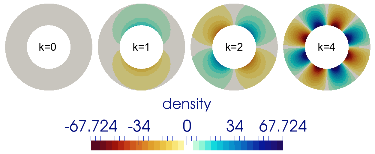
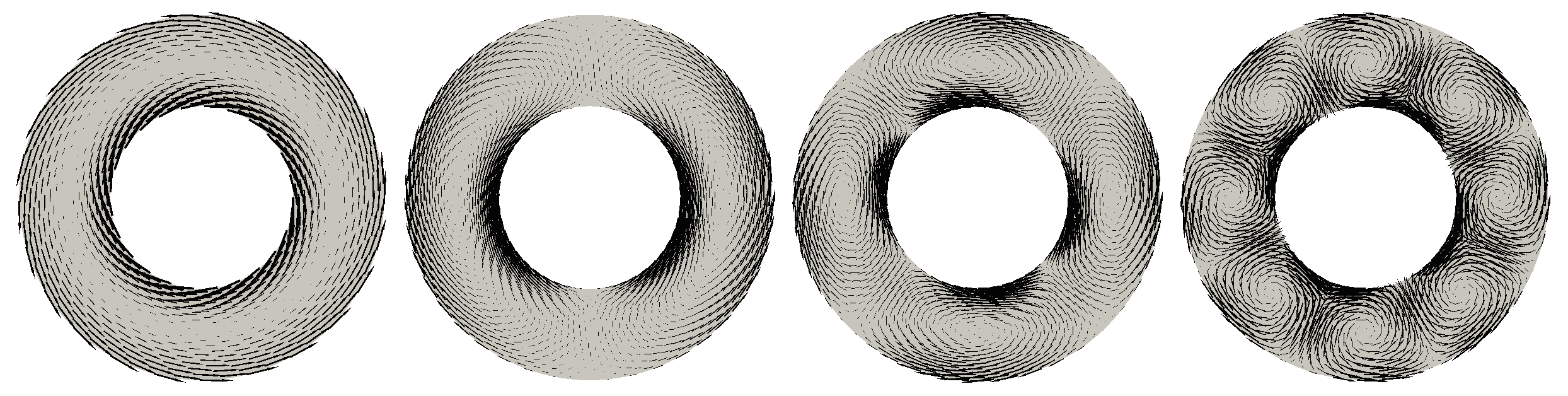
5.4.9 The 2D annulus benchmark

This benchmark is based on Thieulot & Puckett [In prep.] in which an analytical solution to the isoviscous incompressible Stokes equations is derived in an annulus geometry. The velocity and pressure fields are as follows:

\begin{array}{rcl} v_{r} (r, θ) & = & g (r) k sin (k θ), & (71) \\ v_{θ} (r, θ) & = & f (r) cos (k θ), & (72) \\ p (r, θ) & = & k h (r) sin (k θ), & (73) \\ ρ (r, θ) & = & ℵ (r) k sin (k θ), & (74) \end{array}

with

\begin{array}{rcl} f (r) & = & A r + B ∕ r, & (75) \\ g (r) & = & \frac{A}{2} r + \frac{B}{r} ln r + \frac{C}{r}, & (76) \\ h (r) & = & \frac{2 g (r) - f (r)}{r}, & (77) \\ ℵ (r) & = & g^{″} - \frac{g^{'}}{r} - \frac{g}{r^{2}} (k^{2} - 1) + \frac{f}{r^{2}} + \frac{f^{'}}{r}, & (78) \\ A & = & - C \frac{2 (ln R_{1} - ln R_{2})}{R_{2}^{2} ln R_{1} - R_{1}^{2} ln R_{2}}, & (79) \\ B & = & - C \frac{R_{2}^{2} - R_{1}^{2}}{R_{2}^{2} ln R_{1} - R_{1}^{2} ln R_{2}} . & (80) \end{array}

The parameters $A$ and $B$ are chosen so that $v_{r} (R_{1}) = v_{r} (R_{2}) = 0$ , i.e. the velocity is tangential to both inner and outer surfaces. The gravity vector is radial and of unit length.

The parameter $k$ controls the number of convection cells present in the domain, as shown in Fig. 81.

Figure 81: Pressure, density and velocity fields for

k = 0, 1, 2, 3

for the 2D annulus benchmark.

In the present case, we set $R_{1} = 1$ , $R_{2} = 2$ and $C = - 1$ . Fig. 82 shows the velocity and pressure errors in the $L_{2}$ -norm as a function of the mesh size $h$ (taken in this case as the radial extent of the elements). As expected we recover a third-order convergence rate for the velocity and a second-order convergence rate for the pressure.

Figure 82: Velocity and pressure errors in the

L_{2}

-norm as a function of the mesh size for the 2D annulus benchmark.

5.4.10 The “Stokes’ law” benchmark

This section was contributed by Juliane Dannberg.

Stokes’ law was derived by George Gabriel Stokes in 1851 and describes the frictional force a sphere with a density different than the surrounding fluid experiences in a laminar flowing viscous medium. A setup for testing this law is a sphere with the radius $r$ falling in a highly viscous fluid with lower density. Due to its higher density the sphere is accelerated by the gravitational force. While the frictional force increases with the velocity of the falling particle, the buoyancy force remains constant. Thus, after some time the forces will be balanced and the settling velocity of the sphere $v_{s}$ will remain constant:

\begin{align} \underset{frictional force}{\underset{︸}{6 π η r v_{s}}} = \underset{buoyancy force}{\underset{︸}{4 ∕ 3 π r^{3} Δ ρ g,}} & (81) \end{align}

where

η

is the dynamic viscosity of the fluid,

Δ ρ

is the density difference between sphere and fluid and

g

the gravitational acceleration. The resulting settling velocity is then given by

\begin{align} v_{s} = \frac{2}{9} \frac{Δ ρ r^{2} g}{η} . & (82) \end{align}

Because we do not take into account inertia in our numerical computation, the falling particle will reach the constant settling velocity right after the first timestep.

For the setup of this benchmark, we chose the following parameters:

\begin{array}{l} r & = 200 km \\ Δ ρ & = 100 kg ∕ m^{3} \\ η & = 1 0^{22} Pa s \\ g & = 9.81 m ∕ s^{2} . \end{array}

With these values, the exact value of sinking velocity is $v_{s} = 8.72 \cdot 1 0^{- 10} m ∕ s$ .

To run this benchmark, we need to set up an input file that describes the situation. In principle, what we need to do is to describe a spherical object with a density that is larger than the surrounding material. There are multiple ways of doing this. For example, we could simply set the initial temperature of the material in the sphere to a lower value, yielding a higher density with any of the common material models. Or, we could use ASPECT’s facilities to advect along what are called “compositional fields” and make the density dependent on these fields.

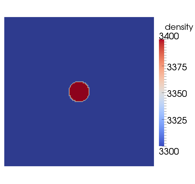
We will go with the second approach and tell ASPECT to advect a single compositional field. The initial conditions for this field will be zero outside the sphere and one inside. We then need to also tell the material model to increase the density by $Δ ρ = 100 k g m^{- 3}$ times the concentration of the compositional field. This can be done, like everything else, from the input file.

All of this setup is then described by the following input file. (You can find the input file to run this cookbook example in cookbooks/stokes.prm. For your first runs you will probably want to reduce the number of mesh refinement steps to make things run more quickly.)

############### Global parameters
# We use a 3d setup. Since we are only interested
# in a steady state solution, we set the end time
# equal to the start time to force a single time
# step before the program terminates.

set ??                              = 3

set ??                             = 0
set ??                               = 0
set ?? = false

set ??                       = output-stokes

############### Parameters describing the model
# The setup is a 3d box with edge length 2890000 in which
# all 6 sides have free slip boundary conditions. Because
# the temperature plays no role in this model we need not
# bother to describe temperature boundary conditions or
# the material parameters that pertain to the temperature.

subsection ??
  set ?? = box

  subsection ??
    set ??  = 2890000
    set ??  = 2890000
    set ??  = 2890000
  end
end

subsection ??
  set ?? = left, right, front, back, bottom, top
end

subsection ??
  set ?? = simple

  subsection ??
    set ??             = 3300
    set ??                     = 1e22
  end
end

subsection ??
  set ?? = vertical

  subsection ??
    set ?? = 9.81
  end
end

############### Parameters describing the temperature field
# As above, there is no need to set anything for the
# temperature boundary conditions.

subsection ??
  set ?? = box
end

subsection ??
  set ?? = function

  subsection ??
    set ?? = 0
  end
end

############### Parameters describing the compositional field
# This, however, is the more important part: We need to describe
# the compositional field and its influence on the density
# function. The following blocks say that we want to
# advect a single compositional field and that we give it an
# initial value that is zero outside a sphere of radius
# r=200000m and centered at the point (p,p,p) with
# p=1445000 (which is half the diameter of the box) and one inside.
# The last block re-opens the material model and sets the
# density differential per unit change in compositional field to
# 100.

subsection ??
  set ?? = 1
end

subsection ??
  set ?? = function

  subsection ??
    set ??      = x,y,z
    set ??  = r=200000,p=1445000
    set ?? = if(sqrt((x-p)*(x-p)+(y-p)*(y-p)+(z-p)*(z-p)) > r, 0, 1)
  end
end

subsection ??
  subsection ??
    set ?? = 100
  end
end

############### Parameters describing the discretization
# The following parameters describe how often we want to refine
# the mesh globally and adaptively, what fraction of cells should
# be refined in each adaptive refinement step, and what refinement
# indicator to use when refining the mesh adaptively.

subsection ??
  set ??        = 4
  set ??          = 4
  set ??                = 0.2
  set ??                           = velocity
end

############### Parameters describing what to do with the solution
# The final section allows us to choose which postprocessors to
# run at the end of each time step. We select to generate graphical
# output that will consist of the primary variables (velocity, pressure,
# temperature and the compositional fields) as well as the density and
# viscosity. We also select to compute some statistics about the
# velocity field.

subsection ??
  set ?? = visualization, velocity statistics

  subsection ??
    set ?? = density, viscosity
  end
end

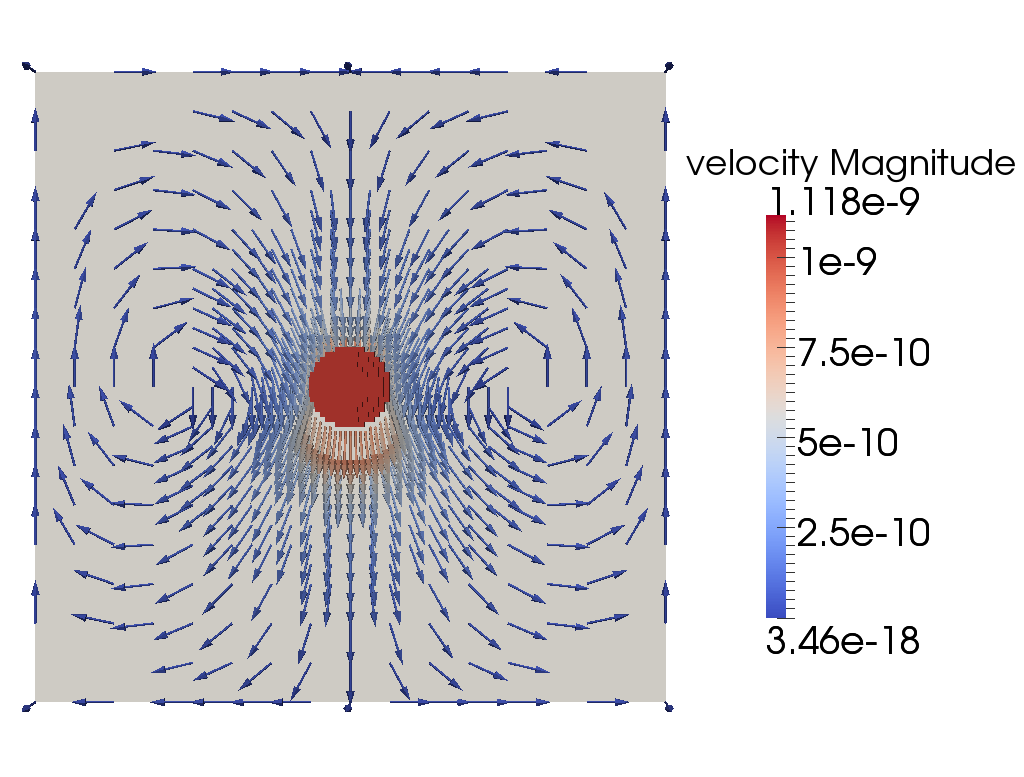
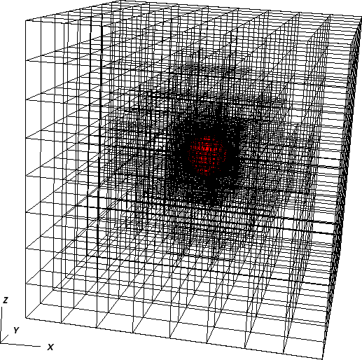
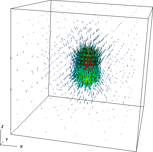
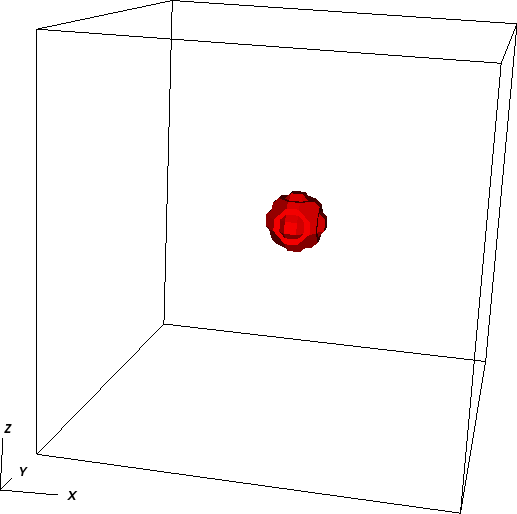
Using this input file, let us try to evaluate the results of the current computations for the settling velocity of the sphere. You can visualize the output in different ways, one of it being ParaView and shown in Fig. 83 (an alternative is to use Visit as described in Section 4.4; 3d images of this simulation using Visit are shown in Fig. 84). Here, Paraview has the advantage that you can calculate the average velocity of the sphere using the following filters:

Threshold (Scalars: C_1, Lower Threshold 0.5, Upper Threshold 1),
Integrate Variables,
Cell Data to Point Data,
Calculator (use the formula sqrt(velocity_x^2+ velocity_y^2+velocity_z^2)/Volume).

If you then look at the Calculator object in the Spreadsheet View, you can see the average sinking velocity of the sphere in the column “Result” and compare it to the theoretical value $v_{s} = 8.72 \cdot 1 0^{- 10} m ∕ s$ . In this case, the numerical result is 8.865 $\cdot 1 0^{- 10} m ∕ s$ when you add a few more refinement steps to actually resolve the 3d flow field adequately. The “velocity statistics” postprocessor we have selected above also provides us with a maximal velocity that is on the same order of magnitude. The difference between the analytical and the numerical values can be explained by different at least the following three points: (i) In our case the sphere is viscous and not rigid as assumed in Stokes’ initial model, leading to a velocity field that varies inside the sphere rather than being constant. (ii) Stokes’ law is derived using an infinite domain but we have a finite box instead. (iii) The mesh may not yet fine enough to provide a fully converges solution. Nevertheless, the fact that we get a result that is accurate to less than 2% is a good indication that ASPECT implements the equations correctly.

Figure 83: Stokes benchmark. Both figures show only a 2D slice of the three-dimensional model. Left: The compositional field and overlaid to it some velocity vectors. The composition is 1 inside a sphere with the radius of 200 km and 0 outside of this sphere. As the velocity vectors show, the sphere sinks in the viscous medium. Right: The density distribution of the model. The compositional density contrast of 100 kg

∕ m^{3}

leads to a higher density inside of the sphere.

Figure 84: Stokes benchmark. Three-dimensional views of the compositional field (left), the adaptively refined mesh (center) and the resulting velocity field (right).

5.4.11 Latent heat benchmark

This section was contributed by Juliane Dannberg.

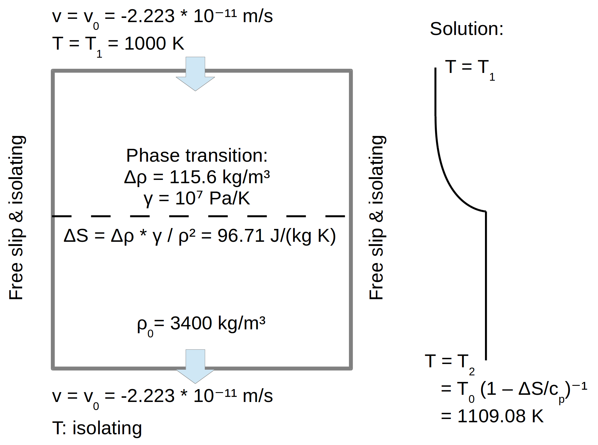
The setup of this benchmark is taken from Schubert, Turcotte and Olson [STO01] (part 1, p. 194) and is illustrated in Fig. 85.

Figure 85: Latent heat benchmark. Both figures show the 2D box model domain. Left: Setup of the benchmark together with a sketch of the expected temperature profile across the phase transition. The dashed line marks the phase transition. Material flows in with a prescribed temperature and velocity at the top, crosses the phase transition in the center and flows out at the bottom. The predicted bottom temperature is

T_{2} = 1109.08 K

. Right: Temperature distribution of the model together with the associated temperature profile across the phase transition. The modelled bottom temperature is

T_{2} = 1107.39 K

It tests whether the latent heat production when material crosses a phase transition is calculated correctly according to the laws of thermodynamics. The material model defines two phases in the model domain with the phase transition approximately in the center. The material flows in from the top due to a prescribed downward velocity, and crosses the phase transition before it leaves the model domain at the bottom. As initial condition, the model uses a uniform temperature field, however, upon the phase change, latent heat is released. This leads to a characteristic temperature profile across the phase transition with a higher temperature in the bottom half of the domain. To compute it, we have to solve equation (3) or its reformulation (5). For steady-state one-dimensional downward flow with vertical velocity $v_{y}$ , it simplifies to the following:

\begin{matrix} ρ C_{p} v_{y} \frac{\partial T}{\partial y} = ρ T Δ S v_{y} \frac{\partial X}{\partial y} + ρ C_{p} κ \frac{\partial^{2} T}{\partial y^{2}} . \end{matrix}

Here, $ρ C_{p} κ = k$ with $k$ the thermal conductivity and $κ$ the thermal diffusivity. The first term on the right-hand side of the equation describes the latent heat produced at the phase transition: It is proportional to the temperature T, the entropy change $Δ S$ across the phase transition divided by the specific heat capacity and the derivative of the phase function X. If the velocity is smaller than a critical value, and under the assumption of a discontinuous phase transition (i.e. with a step function as phase function), this latent heating term will be zero everywhere except for the one point $y_{t r}$ where the phase transition takes place. This means, we have a region above the phase transition with only phase 1, and below a certain depth a jump to a region with only phase 2. Inside of these one-phase regions, we can solve the equation above (using the boundary conditions $T = T_{1}$ for $y \to \infty$ and $T = T_{2}$ for $y \to - \infty$ ) and get

\begin{array}{l} T (y) = \{\begin{matrix} T_{1} + (T_{2} - T_{1}) e^{\frac{v_{y} (y - y_{t r})}{κ}}, & y > y_{t r} \\ T_{2}, & y < y_{t r} \end{matrix} \end{array}

While it is not entirely obvious while this equation for $T (y)$ should be correct (in particular why it should be asymmetric), it is not difficult to verify that it indeed satisfies the equation stated above for both $y < y_{t r}$ and $y > y_{t r}$ . Furthermore, it indeed satisfies the jump condition we get by evaluating the equation at $y = y_{t r}$ . Indeed, the jump condition can be reinterpreted as a balance of heat conduction: We know the amount of heat that is produced at the phase boundary, and as we consider only steady-state, the same amount of heat is conducted upwards from the transition:

\begin{matrix} \underset{latent heat release}{\underset{︸}{ρ v_{y} T Δ S}} = \underset{heat conduction}{\underset{︸}{\frac{κ}{ρ_{0} C_{p}} \frac{\partial T}{\partial y} |_{y = y_{t r^{-}}} = \frac{v_{y}}{ρ_{0} C_{p}} (T_{2} - T_{1})}} \end{matrix}

In contrast to [STO01], we also consider the density change $Δ ρ$ across the phase transition: While the heat conduction takes place above the transition and the density can be assumed as $ρ = ρ_{0} =$ const., the latent heat is released directly at the phase transition. Thus, we assume an average density $ρ = ρ_{0} + 0.5 Δ ρ$ for the left side of the equation. Rearranging this equation gives

\begin{matrix} T_{2} = \frac{T_{1}}{1 - (1 + \frac{Δ ρ}{2 ρ_{0}}) \frac{Δ S}{C_{p}}} \end{matrix}

In addition, we have tested the approach exactly as it is described in [STO01] by setting the entropy change to a specific value and in spite of that using a constant density. However, this is physically inconsistent, as the entropy change is proportional to the density change across the phase transition. With this method, we could reproduce the analytic results from [STO01].

The exact values of the parameters used for this benchmark can be found in Fig. 85. They result in a predicted value of $T_{2} = 1109.08 K$ for the temperature in the bottom half of the model, and we will demonstrate below that we can match this value in our numerical computations. However, it is not as simple as suggested above. In actual numerical computations, we can not exactly reproduce the behavior of Dirac delta functions as would result from taking the derivative $\frac{\partial X}{\partial y}$ of a discontinuous function $X (y)$ . Rather, we have to model $X (y)$ as a function that has a smooth transition from one value to another, over a depth region of a certain width. In the material model plugin we will use below, this depth is an input parameter and we will play with it in the numerical results shown after the input file.

To run this benchmark, we need to set up an input file that describes the situation. In principle, what we need to do is to describe the position and entropy change of the phase transition in addition to the previously outlined boundary and initial conditions. For this purpose, we use the “latent heat” material model that allows us to set the density change $Δ ρ$ and Clapeyron slope $γ$ (which together determine the entropy change via $Δ S = γ \frac{Δ ρ}{ρ^{2}}$ ) as well as the depth of the phase transition as input parameters.

All of this setup is then described by the input file cookbooks/latent-_heat.prm that models flow in a box of $1 0^{6}$ meters of height and width, and a fixed downward velocity. The following section shows the central part of this file:

subsection ??
  set ?? = latent heat
  subsection ??

    # The change of density across the phase transition. Together with the
    # Clapeyron slope, this is what determines the entropy change.
    set ??                 = 115.6
    set ??           = 0

    # If the temperature is equal to the phase transition temperature, the
    # phase transition will occur at the phase transition depth. However,
    # if the temperature deviates from this value, the Clapeyron slope
    # determines how much the pressure (and depth) of the phase boundary
    # changes. Here, the phase transition will be in the middle of the box
    # for T=T1.
    set ??                        = 500000
    set ??                  = 1000
    set ??              = 1e7

    # We set the width of the phase transition to 5 km. You may want to
    # change this parameter to see how latent heating depends on the width
    # of the phase transition.
    set ??                        = 5000

    set ??                              = 3400
    set ??                        = 1000
    set ??                          = 1000
    set ??                           = 2.38

    # We set the thermal expansion amd the compressibility to zero, so that
    # all temperature (and density) changes are caused by advection, diffusion
    # and latent heating.
    set ??                  = 0.0
    set ??                                = 0.0

    # Viscosity is constant.
    set ??                     = 0.0
    set ??                                      = 8.44e21
    set ??                           = 1.0, 1.0
    set ??                = 1.0
  end
end

The complete input file referenced above also sets the number of mesh refinement steps. For your first runs you will probably want to reduce the number of mesh refinement steps to make things run more quickly. Later on, you might also want to change the phase transition width to look how this influences the result.

Figure 86: Results of the latent heat benchmark. Both figures show the modelled temperature

T_{2}

at the bottom of the model domain. Left:

T_{2}

in dependence of resolution using a constant phase transition width of 20km. With an increasing number of global refinements of the mesh, the bottom temperature converges against a value of

T_{2} = 1105.27 K

. Right:

T_{2}

in dependence of phase transition width. The model resolution is chosen proportional to the phase transition width, starting with 5 global refinements for a width of 20km. With decreasing phase transition width,

T_{2}

approaches the theoretical value of

1109.08 K

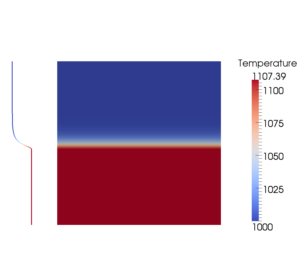
Using this input file, let us try to evaluate the results of the current computations. We note that it takes some time for the model to reach a steady state and only then does the bottom temperature reach the theoretical value. Therefore, we use the last output step to compare predicted and computed values. You can visualize the output in different ways, one of it being ParaView and shown in Fig. 85 on the right side (an alternative is to use Visit as described in Section 4.4). 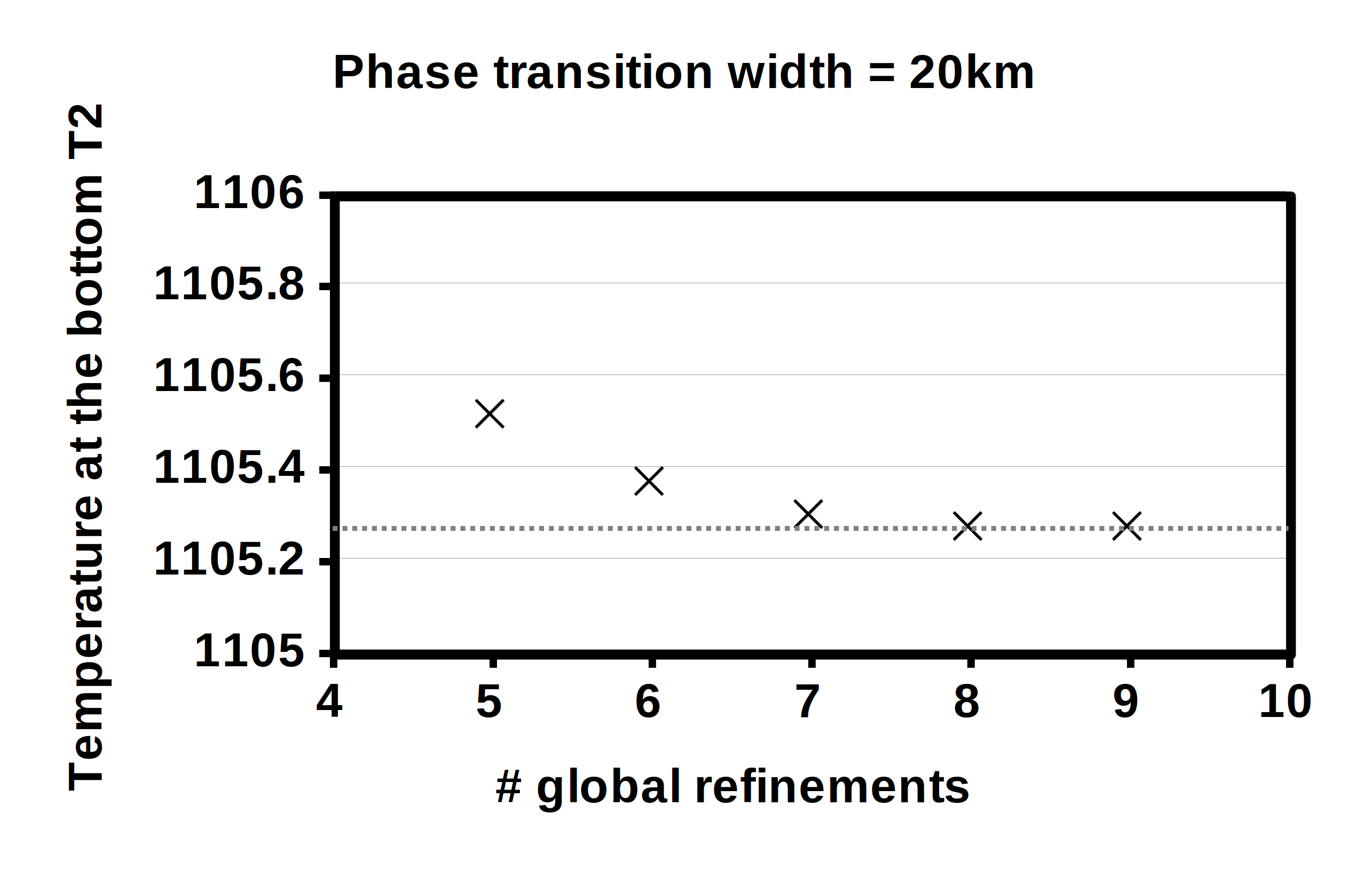In ParaView, you can plot the temperature profile using the filter “Plot Over Line” (Point1: 500000,0,0; Point2: 500000,1000000,0, then go to the “Display” tab and select “T” as only variable in the “Line series” section) or “Calculator” (as seen in Fig. 85). In Fig. 86 (left) we can see that with increasing resolution, the value for the bottom temperature converges to a value of $T_{2} = 1105.27 K$ .

However, this is not what the analytic solution predicted. The reason for this difference is the width of the phase transition with which we smooth out the Dirac delta function that results from differentiating the $X (y)$ we would have liked to use in an ideal world. (In reality, however, for the Earth’s mantle we also expect phase transitions that are distributed over a certain depth range and so the smoothed out approach may not be a bad approximation.) Of course, the results shown above result from an the analytical approach that is only correct if the phase transition is discontinuous and constrained to one specific depth $y = y_{t r}$ . 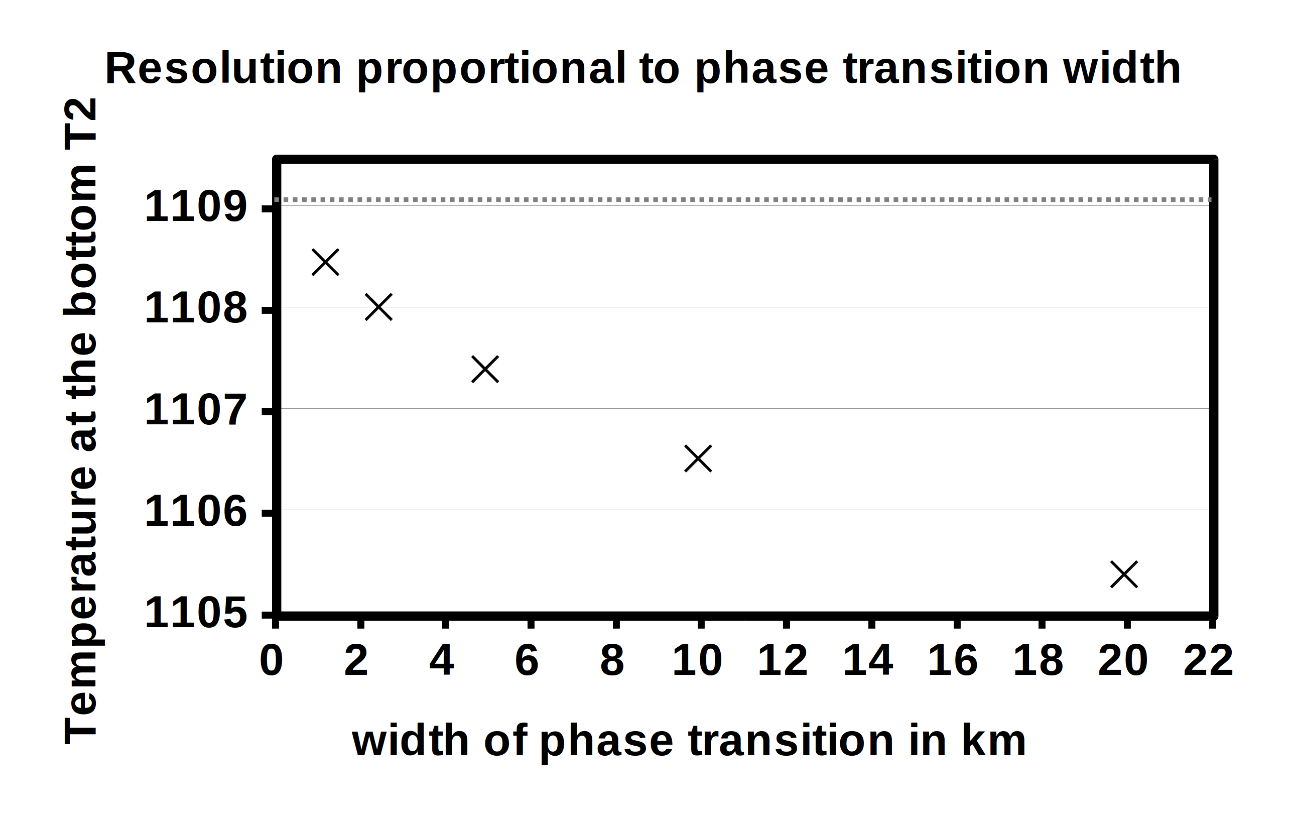Instead, we chose a hyperbolic tangent as our phase function. Moreover, Fig. 86 (right) illustrates what happens to the temperature at the bottom when we vary the width of the phase transition: The smaller the width, the closer the temperature gets to the predicted value of $T_{2} = 1109.08 K$ , demonstrating that we converge to the correct solution.

5.4.12 The 2D cylindrical shell benchmarks by Davies et al.

This section was contributed by William Durkin and Wolfgang Bangerth.

All of the benchmarks presented so far take place in a Cartesian domain. Davies et al. describe a benchmark (in a paper that is currently still being written) for a 2D spherical Earth that is nondimensionalized such that

$r_{min}$ = 1.22	${T\|}_{r_{m i n}}$ = 1
$r_{max}$ = 2.22	${T\|}_{r_{m a x}}$ = 0

The benchmark is run for a series of approximations (Boussinesq, Extended Boussinesq, Truncated Anelastic Liquid, and Anelastic Liquid), and temperature, velocity, and heat flux calculations are compared with the results of other mantle modeling programs. ASPECT will output all of these values directly except for the Nusselt number, which we must calculate ourselves from the heat fluxes that ASPECT can compute. The Nusselt number of the top and bottom surfaces, ${N u}_{T}$ and ${N u}_{B}$ , respectively, are defined by the authors of the benchmarks as

{N u}_{T} = \frac{ln (f)}{2 π r_{max} (1 - f)} \int_{0}^{2 π} \frac{\partial T}{\partial r} d θ

(83)

and

{N u}_{B} = \frac{f ln (f)}{2 π r_{min} (1 - f)} \int_{0}^{2 π} \frac{\partial T}{\partial r} d θ

where $f$ is the ratio $\frac{r_{min}}{r_{max}}$ .

We can put this in terms of heat flux

q_{r} = - k \frac{\partial T}{\partial r}

through the inner and outer surfaces, where $q_{r}$ is heat flux in the radial direction. Let $Q$ be the total heat that flows through a surface,

Q = \int_{0}^{2 π} q_{r} d θ,

then (83) becomes

{N u}_{T} = \frac{- Q_{T} ln (f)}{2 π r_{max} (1 - f) k}

and similarly

{N u}_{B} = \frac{- Q_{B} f ln (f)}{2 π r_{min} (1 - f) k} .

$Q_{T}$ and $Q_{B}$ are heat fluxes that ASPECT can readily compute through the heat flux statistics postprocessor (see Section ??). For further details on the nondimensionalization and equations used for each approximation, refer to Davies et al.

The series of benchmarks is then defined by a number of cases relating to the exact equations chosen to model the fluid. We will discuss these in the following.

Case 1.1: BA_Ra104_Iso_ZS. This case is run with the following settings:

Boussinesq Approximation
Boundary Condition: Zero-Slip
Rayleigh Number = $1 0^{4}$
Initial Conditions: $D = 0, O = 4$
$η (T) = 1$

where $D$ and $O$ refer to the degree and order of a spherical harmonic that describes the initial temperature. While the initial conditions matter, what is important here though is that the system evolve to four convective cells since we are only interested in the long term, steady state behavior.

The model is relatively straightforward to set up, basing the input file on that discussed in Section 5.3.1. The full input file can be found at benchmarks/davies_et_al/case-_1.1.prm, with the interesting parts excerpted as follows:

############### Parameters describing the model

subsection ??
  set ?? = spherical shell
  subsection ??
    set ??  = 1.22
    set ?? = 360
    set ??  = 2.22
  end
end

# [...]

subsection ??
  set ?? = simple
  subsection ??
    set ??             = 1
    set ??       = 1.
    set ??         = 0
    set ??          = 1
    set ?? = 1e-6
    set ??                     = 1
  end
end

############### Parameters describing the temperature field
# Angular mode is set to 4 in order to match the number of
# convective cells reported by Davies et al.

subsection ??
  set ?? = spherical hexagonal perturbation
  subsection ??
    set ??          = 4
    set ??       = 0
  end
end

############### Prescribe the Rayleigh number as g*alpha
# Here, Ra = 10^4 and alpha was chosen as 10^-6 above.
subsection ??
  set ?? = radial constant
  subsection ??
    set ?? =  1e10
  end
end

# [...]

We use the same trick here as in Section 5.2.1 to produce a model in which the density $ρ (T)$ in the temperature equation (3) is almost constant (namely, by choosing a very small thermal expansion coefficient) as required by the benchmark, and instead prescribe the desired Rayleigh number by choosing a correspondingly large gravity.

Results for this and the other cases are shown below.

Case 2.1: BA_Ra104_Iso_FS. Case 2.1 uses the following setup, differing only in the boundary conditions:

Boussinesq Approximation
Boundary Condition: Free-Slip
Rayleigh Number = $1 0^{4}$
Initial Conditions: $D = 0, O = 4$
$η (T) = 1$

As a consequence of the free slip boundary conditions, any solid body rotation of the entire system satisfies the Stokes equations with their boundary conditions. In other words, the solution of the problem is not unique: given a solution, adding a solid body rotation yields another solution. We select arbitrarily the one that has no net rotation (see Section ??). The section in the input file that is relevant is then as follows (the full input file resides at benchmarks/davies_et_al/case-_2.1.prm):

subsection ??
  set ??                        = net rotation
end

subsection ??
  set ??   = 0,1
end

subsection ??
  set ?? = 0,1
end

Again, results are shown below.

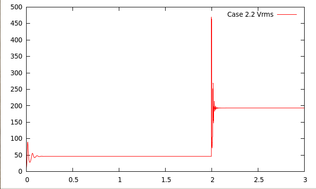
Case 2.2: BA_Ra105_Iso_FS. Case 2.2 is described as follows:

Boussinesq Approximation
Boundary Condition: Free-Slip
Rayleigh Number = $1 0^{5}$
Initial Conditions: Final conditions of case 2.1 (BA_Ra104_Iso_FS)
$η (T) = 1$

In other words, we have an increased Rayleigh number and begin with the final steady state of case 2.1. To start the model where case 2.1 left off, the input file of case 2.1, benchmarks/davies_et_al/case-_2.1.prm, instructs ASPECT to checkpoint itself every few time steps (see Section 4.5). If case 2.2 uses the same output directory, we can then resume the computations from this checkpoint with an input file that prescribes a different Rayleigh number and a later input time:

############### Global parameters
# Case 2.2 begins with the final steady state solution of Case 2.1
# "Resume computation" must be set to true, and "Output directory" must
# point to the folder that contains the results of Case 2.1.

set ??                             = 10

set ??                               = 3
set ??                       = output

set ??                     = true

We increase the Rayleigh number to $1 0^{5}$ by increasing the magnitude of gravity in the input file. The full script for case 2.2 is located in benchmarks/davies_et_al/case-_2.2.prm

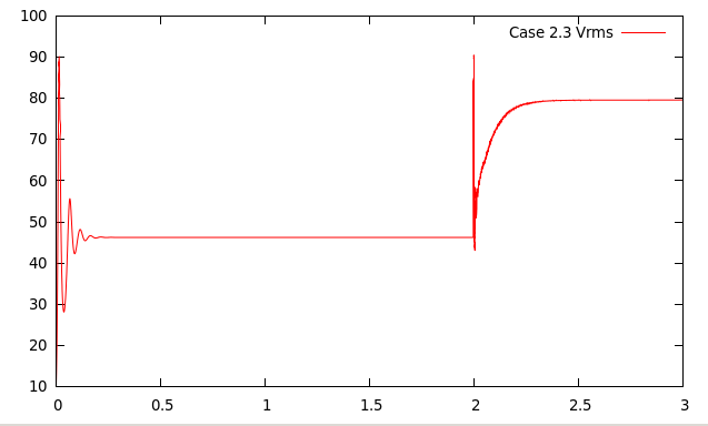
Case 2.3: BA_Ra103_vv_FS. Case 2.3 is a variation on the previous one:

Boussinesq Approximation
Boundary Condition: Free-Slip
Rayleigh Number = $1 0^{3}$
Initial Conditions: Final conditions of case 2.1 (BA_Ra104_Iso_FS)
$η (T) = 100 0^{- T}$

The Rayleigh number is smaller here (and is selected using the gravity parameter in the input file, as before), but the more important change is that the viscosity is now a function of temperature. At the time of writing, there is no material model that would implement such a viscosity, so we create a plugin that does so for us (see Sections 6 and 6.2 in general, and Section 6.3.1 for material models in particular). The code for it is located in benchmarks/davies_et_al/case-_2.3-_plugin/VoT.cc (where “VoT” is short for “viscosity as a function of temperature”) and is essentially a copy of the simpler material model. The primary change compared to the simpler material model is the line about the viscosity in the following function:

template <int dim>
void
VoT<dim>::
evaluate(const typename Interface<dim>::MaterialModelInputs &in,
         typename Interface<dim>::MaterialModelOutputs &out) const
{
  for (unsigned int i=0; i<in.position.size(); ++i)
    {
      out.viscosities[i] = eta*std::pow(1000,(-in.temperature[i]));
      out.densities[i] = reference_rho * (1.0 - thermal_alpha * (in.temperature[i] - reference_T));
      out.thermal_expansion_coefficients[i] = thermal_alpha;
      out.specific_heat[i] = reference_specific_heat;
      out.thermal_conductivities[i] = k_value;
      out.compressibilities[i] = 0.0;
    }
}

Using the method described in Sections 5.4.1 and 6.2, and the files in the benchmarks/davies_et_al/case-2.3-plugin, we can compile our new material model into a shared library that we can then reference from the input file. The complete input file for case 2.3 is located in benchmarks/davies_et_al/case-_2.3.prm and contains among others the following parts:

set ??            = ./case-2.3-plugin/libVoT.so

subsection ??
  set ?? = VoT

  subsection ??
    set ??             = 1
    set ??       = 1.
    set ??         = 0
    set ??          = 1
    set ?? = 1e-5
    set ??                     = 1
  end
end

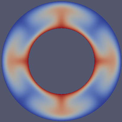
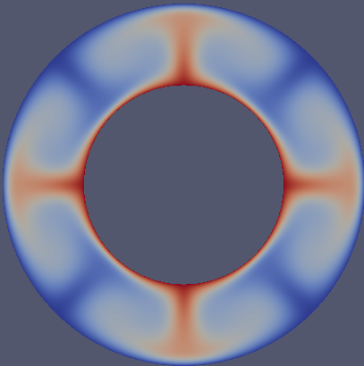
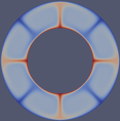
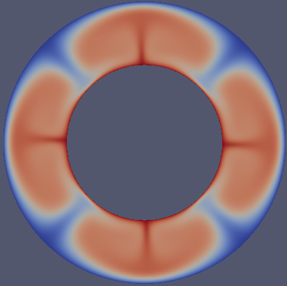
Results. In the following, let us discuss some of the results of the benchmark setups discussed above. First, the final steady state temperature fields are shown in Fig. 87. It is immediately obvious how the different Rayleigh numbers affect the width of the plumes. If one imagines a setup with constant gravity, constant inner and outer temperatures and constant thermal expansion coefficient (this is not how we describe it in the input files, but we could have done so and it is closer to how we intuit about fluids than adjusting the gravity), then the Rayleigh number is inversely proportional to the viscosity – and it is immediately clear that larger Rayleigh numbers (corresponding to lower viscosities) then lead to thinner plumes. This is nicely reflected in the visualizations.

(a) Case 1.1

(b) Case 2.1

(d) Case 2.3

Figure 87: Davies et al. benchmarks: Final steady state temperature fields for the 2D cylindrical benchmark cases.

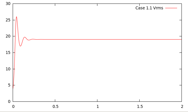
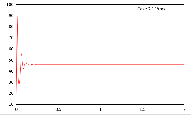
Secondly, Fig. 88 shows the root mean square velocity as a function of time for the various cases. It is obvious that they all converge to steady state solutions. However, there is an initial transient stage and, in cases 2.2 and 2.3, a sudden jolt to the system at the time where we switch from the model used to compute up to time $t = 2$ to the different models used after that.

(a) Case 1.1

(b) Case 2.1

(d) Case 2.3

Figure 88: Davies et al. benchmarks:

V_{rms}

for 2D Cylindrical Cases. Large jumps occur when transitioning from case 2.1 to cases 2.2 and 2.3 due to the instantaneous change of parameter settings.

These runs also produce quantitative data that will be published along with the concise descriptions of the benchmarks and a comparison with other codes. In particular, some of the criteria listed above to judge the accuracy of results are listed in Table 7.³⁶


Case	$<T>$	$N u_{T}$	$N u_{B}$	$V_{rms}$

1.1	0.403	2.464	2.468	19.053
2.1	0.382	4.7000	4.706	46.244
2.2	0.382	9.548	9.584	193.371
2.3	0.582	5.102	5.121	79.632

Table 7: Davies et al. benchmarks: Numerical results for some of the output quantities required by the benchmarks and the various cases considered.

5.4.13 The Crameri et al. benchmarks

This section was contributed by Ian Rose.

This section follows the two free surface benchmarks described by Crameri et al. [CSG $^{+}$ 12].

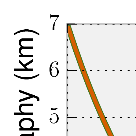
Case 1: Relaxation of topography. The first benchmark involves a high viscosity lid sitting on top of a lower viscosity mantle. There is an initial sinusoidal topography which is then allowed to relax. This benchmark has a semi-analytical solution (which is exact for infinitesimally small topography). Details for the benchmark setup are in Figure 89.

Figure 89: Setup for the topography relaxation benchmark. The box is

2800

km wide and

700

km high, with a

100

km lid on top. The lid has a viscosity of

1 0^{23} P a s

, while the mantle has a viscosity of

1 0^{21} P a s

. The sides are free slip, the bottom is no slip, and the top is a free surface. Both the lid and the mantle have a density of

3300 k g ∕ m^{3}

, and gravity is

10 m ∕ s^{2}

. There is a

7 k m

sinusoidal initial topography on the free surface.

The complete parameter file for this benchmark can be found in benchmarks/crameri_et_al/case_1/crameri_benchmark_1.prm, the most relevant parts of which are excerpted here:

set CFL number                             = 0.01

set Additional shared libraries = ./libcrameri_benchmark_1.so

subsection Geometry model
  set Model name = rebound box
  subsection Rebound Box
    set Order = 1
    set Amplitude = 7.e3
  end
  subsection Box
    set X extent = 28.e5
    set Y extent = 7.e5
    set X repetitions = 300
    set Y repetitions = 75
  end
end

In particular, this benchmark uses a custom geometry model to set the initial geometry. This geometry model, called “ReboundBox”, is based on the Box geometry model. It generates a domain in using the same parameters as Box, but then displaces all the nodes vertically with a sinusoidal perturbation, where the magnitude and order of that perturbation are specified in the ReboundBox subsection.

The characteristic timescales of topography relaxation are significantly smaller than those of mantle convection. Taking timesteps larger than this relaxation timescale tends to cause sloshing instabilities, which are described further in Section 2.12. Some sort of stabilization is required to take large timesteps. In this benchmark, however, we are interested in the relaxation timescale, so we are free to take very small timesteps (in this case, 0.01 times the CFL number). As can be seen in Figure 90, the results of all the codes which are included in this comparison are basically indistinguishable.

Figure 90: Results for the topography relaxation benchmark, showing maximum topography versus time. Over about

100

ka the topography completely disappears. The results of four free surface codes, as well as the semi-analytic solution, are nearly identical.

Case 2: Dynamic topography. Case two is more complicated. Unlike the case one, it occurs over mantle convection timescales. In this benchmark there is the same high viscosity lid over a lower viscosity mantle. However, now there is a blob of buoyant material rising in the center of the domain, causing dynamic topography at the surface. The details for the setup are in the caption of Figure 91.

Figure 91: Setup for the dynamic topography benchmark. Again, the domain is

2800

km wide and

700

km high. A

100

km thick lid with viscosity

1 0^{23}

overlies a mantle with viscosity

1 0^{21}

. Both the lid and the mantle have a density of

3300 k g ∕ m^{3}

. A blob with diameter

100

km lies

300

km from the bottom of the domain. The blob has a density of

3200 k g ∕ m^{3}

and a viscosity of

1 0^{20}

Pa s.

Case two requires higher resolution and longer time integrations than case one. The benchmark is over 20 million years and builds dynamic topography of $\sim 800$ meters.

Figure 92: Evolution of topography for the dynamic topography benchmark. The maximum topography is shown as a function of time, for ASPECT as well as for several other codes participating in the benchmark. This benchmark shows considerably more scatter between the codes.

Again, we excerpt the most relevant parts of the parameter file for this benchmark, with the full thing available in benchmarks/crameri_et_al/case_2/crameri_benchmark_2.prm. Here we use the “Multicomponent” material model, which allows us to easily set up a number of compositional fields with different material properties. The first compositional field corresponds to background mantle, the second corresponds to the rising blob, and the third corresponds to the viscous lid.

Furthermore, the results of this benchmark are sensitive to the mesh refinement and timestepping parameters. Here we have nine refinement levels, and refine according to density and the compositional fields.

set CFL number                   = 0.1

subsection Material model
  set Model name = multicomponent
  subsection Multicomponent
    set Densities = 3300, 3200, 3300
    set Viscosities = 1.e21, 1.e20, 1.e23
    set Viscosity averaging scheme = harmonic
  end
end

subsection Mesh refinement
  set Additional refinement times        =
  set Initial adaptive refinement        = 4
  set Initial global refinement          = 5
  set Refinement fraction                = 0.3
  set Coarsening fraction                = 0.0
  set Strategy                           = density,composition
  set Refinement criteria merge operation = plus
  set Time steps between mesh refinement = 5
end

Unlike the first benchmark, for case two there is no (semi) analytical solution to compare against. Furthermore, the time integration for this benchmark is much longer, allowing for errors to accumulate. As such, there is considerably more scatter between the participating codes. ASPECT does, however, fall within the range of the other results, and the curve is somewhat less wiggly. The results for maximum topography versus time are shown in 92

The precise values for topography at a given time are quite dependent on the resolution and timestepping parameters. Following [CSG $^{+}$ 12] we investigate the convergence of the maximum topography at 3 Ma as a function of CFL number and mesh resolution. The results are shown in figure 93.

Figure 93: Convergence for case two. Left: Logarithm of the error with decreasing CFL number. As the CFL number decreases, the error gets smaller. However, once it reaches a value of

\sim 0.1

, there stops being much improvement in accuracy. Right: Logarithm of the error with increasing maximum mesh resolution. As the resolution increases, so does the accuracy.

We find that at 3 Ma ASPECT converges to a maximum topography of $\sim$ 396 meters. This is slightly different from what MILAMIN_VEP reported as its convergent value in [CSG $^{+}$ 12], but still well within the range of variation of the codes. Additionally, we note that ASPECT is able to achieve good results with relatively less mesh resolution due to the ability to adaptively refine in the regions of interest (namely, the blob and the high viscosity lid).

Accuracy improves roughly linearly with decreasing CFL number, though stops improving at CFL $\sim 0.1$ . Accuracy also improves with increasing mesh resolution, though its convergence order does not seem to be excellent. It is possible that other mesh refinement parameters than we tried in this benchmark could improve the convergence. The primary challenge in accuracy is limiting numerical diffusion of the rising blob. If the blob becomes too diffuse, its ability to lift topography is diminished. It would be instructive to compare the results of this benchmark using particles with the results using compositional fields.

5.4.14 The solitary wave benchmark

This section was contributed by Juliane Dannberg and is based on a section in [DH16] by Juliane Dannberg and Timo Heister.

One of the most widely used benchmarks for codes that model the migration of melt through a compacting and dilating matrix is the propagation of solitary waves (e.g. [SS11, KMK13, Sch00]). The benchmark is intended to test the accuracy of the solution of the two-phase flow equations as described in Section 2.13 and makes use of the fact that there is an analytical solution for the shape of solitary waves that travel through a partially molten rock with a constant background porosity without changing their shape and with a constant wave speed. Here, we follow the setup of the benchmark as it is described in [BR86], which considers one-dimensional solitary waves.

The model features a perturbation of higher porosity with the amplitude $A ϕ_{0}$ in a uniform low-porosity ( $ϕ = ϕ_{0}$ ) background. Due to its lower density, melt migrates upwards, dilating the solid matrix at its front and compacting it at its end.

Assuming constant shear and compaction viscosities and using a permeability law of the form

\begin{array}{l} k_{ϕ} & = k_{0} ϕ^{3}, & implying a Darcy coefficient K_{D} (ϕ) = \frac{k_{0}}{η_{f}} ϕ^{3}, \\ and the non-dimensionalization \\ x & = δ x^{'} & with the compaction length δ = \sqrt{K_{D} (ϕ_{0}) (ξ + \frac{4}{3} η)}, \\ ϕ & = ϕ_{0} ϕ^{'} & with the background porosity ϕ_{0}, \\ (u_{s}, u_{f}) & = u_{0} {(u_{s}, u_{f})}^{'} & with the separation flux ϕ_{0} u_{0} = K_{D} (ϕ_{0}) Δ ρ g, \end{array}

the analytical solution for the shape of the solitary wave can be written in implicit form as:

\begin{array}{l} x (ϕ) & = \pm (A + 0.5) [- 2 \sqrt{A - ϕ} + \frac{1}{\sqrt{A - 1}} ln \frac{\sqrt{A - 1} - \sqrt{A - ϕ}}{\sqrt{A - 1} + \sqrt{A - ϕ}}] \end{array}

and the phase speed $c$ , scaled back to physical units, is $c = u_{0} (2 A + 1)$ . This is only valid in the limit of small porosity $ϕ_{0} « 1$ . Figure 94 illustrates the model setup.

Figure 94: Setup of the solitary wave benchmark. The domain is

400

m high and includes a low porosity (

ϕ = 0.001

) background with an initial perturbation (

ϕ = 0.1

). The solid density is

3300 k g ∕ m^{3}

and the melt density is

2500 k g ∕ m^{3}

. We apply the negative phase speed of the solitary wave

u_{s} = - c e_{z}

as velocity boundary condition, so that the wave will stay at its original position while the background is moving.

The parameter file and material model for this setup can be found in benchmarks/solitary_wave/solitary_wave.prm and benchmarks/solitary_wave/solitary_wave.cc. The most relevant sections are shown in the following paragraph.

# Listing of Parameters
# ---------------------
# Set up the solitary wave benchmark
# (Barcilon & Richter, 1986; Simpson & Spiegelman, 2011;
# Keller et al., 2013; Schmeling, 200

set Additional shared libraries            = ./libsolitary_wave.so

# A non-linear solver has to be used for models with melt migration
set Nonlinear solver scheme                = iterated Advection and Stokes
set Max nonlinear iterations               = 10
set Nonlinear solver tolerance             = 1e-5

# The end time is chosen in such a way that the solitary wave travels
# approximately 5 times its wavelength during the model time.
set End time                               = 6e6

# To model melt migration, there has to be a compositional field with
# the name ’porosity’.
subsection Compositional fields
  set Number of fields = 1
  set Names of fields = porosity
end

# Enable modelling of melt migration in addition to the advection of
# solid material.
subsection Melt settings
  set Include melt transport                  = true
end

######### Parameters for the porosity field ########################

# We use the initial conditions and material model from the
# solitary wave plugin and choose a wave with an amplitude of
# 0.01 and a background porosity of 0.001.
subsection Initial composition model
  set Model name = Solitary wave initial condition
  subsection Solitary wave initial condition
    set Offset = 200
    set Read solution from file = true
    set Amplitude = 0.01
    set Background porosity = 0.001
  end
end

subsection Material model
  set Model name = Solitary Wave
end

# As material is flowing in, we prescribe the porosity at the
# upper and lower boundary.
subsection Boundary composition model
  set List of model names = initial composition
  set Fixed composition boundary indicators   = 2,3
end

# As we know that our solution does not have any steep gradients
# we can use a low stabilization to avoid too much diffusion.
subsection Discretization
  subsection Stabilization parameters
    set beta  = 0.001
  end
end

######### Model geometry ##############################################

# Our domain is a pseudo-1D-profile 400 m in height, but only a few elements wide
subsection Geometry model
  set Model name = box
  subsection Box
    set X extent  = 10
    set Y extent  = 400
    set Y repetitions = 40
  end
end

######### Velocity boundary conditions ################################

# We apply the phase speed of the wave here, so that it always stays in the
# same place in our model. The phase speed is c = 5.25e-11 m/s, but we have
# to convert it to m/years using the same conversion that is used internally
# in Aspect: year_in_seconds = 60*60*24*365.2425.
subsection Boundary velocity model
  set Tangential velocity boundary indicators = 0,1
  set Prescribed velocity boundary indicators = 2:function, 3:function
  subsection Function
    set Function expression = 0;-1.65673998e-4
  end
end

# Postprocessor for the error calculation
subsection Postprocess
  set List of postprocessors = solitary wave statistics
end

subsection Solver parameters
  subsection Stokes solver parameters
    set Linear solver tolerance = 1e-10
  end
end

The benchmark uses a custom model to generate the initial condition for the porosity field as specified by the analytical solution, and its own material model, which includes the additional material properties needed by models with melt migration, such as the permeability, melt density and compaction viscosity. The solitary wave postprocessor compares the porosity and pressure in the model to the analytical solution, and computes the errors for the shape of the porosity, shape of the compaction pressure and the phase speed. We apply the negative phase speed of the solitary wave as a boundary condition for the solid velocity. This changes the reference frame, so that the solitary wave stays in the center of the domain, while the solid moves downwards. The temperature evolution does not play a role in this benchmark, so all temperature and heating-related parameters are disabled or set to zero.

And extensive discussion of the results and convergence behavior can be found in [DH16].

5.4.15 Benchmarks for operator splitting

This section was contributed by Juliane Dannberg.

Models of mantle convection and lithosphere dynamics often also contain reactions between materials with different chemical compositions, or processes that can be described as reactions. The most common example is mantle melting: When mantle temperatures exceed the solidus, rocks start to melt. As this is only partial melting, and rocks are a mixture of different minerals, which all contain different chemical components, melting is not only a phase transition, but also leads to reactions between solid and molten rock. Some components are more compatible with the mineral structure, and preferentially stay in the solid rock, other components will mainly move into the mantle melt. This means that the composition of both solid and melt change over time depending on the melt fraction.

Usually, it is assumed that these reactions are much faster than convection in the mantle. In other words, these reactions are so fast that melt is assumed to be always in equilibrium with the surrounding solid rock. In some cases, the formation of new oceanic crust, which is also caused by partial melting, is approximated by a conversion from an average, peridotitic mantle composition to mid-ocean ridge basalt, forming the crust, and harzburgitic lithosphere, once material reaches a given depth. This process can also be considered as a reaction between different compositional fields.

This can cause accuracy problems in geodynamic simulations: The way the equations are formulated (see Equations 1–4), ideally we would need to know reaction rates (the $q_{i}$ ) between the different components instead of the equilibrium value (which would then have to be compared with some sort of “old solution” of the compositional fields). Sometimes we also may not know the equilibrium, and would only be able to find it iteratively, starting from the current composition. In addition, the reaction rate for a given compositional field usually depends on the value of the field itself, but can also depend on other compositional fields or the temperature and pressure, and the dependence can be nonlinear.

Hence, ASPECT has the option to decouple the advection from reactions between compositional fields, using operator splitting.

Instead of solving the coupled equation

\begin{align} \frac{\partial c (t)}{\partial t} + u \cdot \nabla c (t) & = q (c (t)), & (84) \end{align}

and directly obtaining the composition value $c (t^{n + 1})$ for the time step $n + 1$ from the value $c (t^{n})$ from the previous time step $n$ , we do a first-order operator split, first solving the advection problem

\begin{align} \frac{\partial c (t)}{\partial t} + u \cdot \nabla c (t) & = 0, & obtaining Δ c_{A} (t^{n + 1}) from c (t^{n}), & (85) \end{align}

using the advection time step $Δ t_{A} = t^{n + 1} - t^{n}$ . Then we solve the reactions as a series of coupled ordinary differential equations

\begin{align} \frac{\partial Δ c_{R} (t)}{\partial t} & = q (c (t^{n})) + Δ c_{A} (t^{n + 1}) + Δ c_{R} (t), & obtaining Δ c_{R} (t^{n + 1}) from c (t^{n}) + Δ c_{A} (t^{n + 1}) . & (86) \end{align}

This can be done in several iterations, choosing a different, smaller time step size $Δ t_{R} \leq Δ t_{A}$ for the time discretization. The updated value of the compositional field after the overall (advection + reaction) time step is then obtained as

\begin{align} c (t^{n + 1}) & = c (t^{n}) + Δ c_{A} (t^{n + 1}) + Δ c_{R} (t^{n + 1}) . & (87) \end{align}

This is very useful if the time scales of reactions are different from the time scales of convection. The same scheme can also be used for the temperature: If we want to model latent heat of melting, the temperature evolution is controlled by the melting rate, and hence the temperature changes on the same time scale as the reactions.

We here illustrate the way this operator splitting works using the simple example of exponential decay in a stationary advection field. We will start with a model that has a constant initial temperature and composition and no advection. The reactions for exponential decay

\begin{align} c (t) & = c_{0} e^{λ t} with λ = - log (2) ∕ t_{1 ∕ 2}, & (88) \end{align}

where $c_{0}$ is the initial composition and $t_{1 ∕ 2}$ is the half life, are implemented in a shared library (benchmarks/operator_splitting/exponential_decay/exponential_decay.cc). As we split the time-stepping of advection and reactions, there are now two different time steps in the model: We control the advection time step using the ‘Maximum time step’ parameter (as the velocity is essentially 0, we can not use the CFL number), and we set the reaction time step using the ‘Reaction time step’ parameter.

set ?? = ./libexponential_decay.so

set ??                              = 2
set ??                             = 0
set ??                               = 100

# We use a new solver scheme otpion that enables the operator split.
set ??                = single Advection, single Stokes
set ??                 = true

subsection ??
  subsection ??
    set ??                 = 0.0005
  end
end
set ??                      = 10

To illustrate convergence, we will vary both parameters in different model runs.

In our example, we choose $c_{0} = 1$ , and specify this as initial condition using the function plugin for both composition and temperature. We also set $t_{1 ∕ 2} = 10$ , which is implemented as a parameter in the exponential decay material model and the exponential decay heating model.

# Both initial temperature and composition are set to 1,
# and will decay starting from this value.
subsection ??
  set ?? = function

  subsection ??
    set ??      = x,z
    set ?? = 1.0
  end
end

subsection ??
  set ?? = function

  subsection ??
    set ??      = x,z
    set ?? = 1.0
  end
end

# We choose material and heating models that let temperature
# and composition decay over time, and that is implemented in
# a plugin.
subsection ??
  set ?? = exponential decay heating

  subsection ??
    set ?? = 10
  end
end

subsection ??
  set ?? = exponential decay

  subsection ??
    set ?? = 10
  end
end

The complete parameter file for this setup can be found in benchmarks/operator_splitting/exponential_decay/exponential_decay.base.prm.

Figure 95 shows the convergence behavior of these models: As there is no advection, the advection time step does not influence the error (blue data points). As we use a first-order operator split, the error is expected to converge linearly with the reaction time step $Δ t_{R}$ , which is indeed the case (red data points). Errors are the same for both composition and temperature, as both fields have identical initial conditions and reactions, and we use the same methods to solve for these variables.

Figure 95: Error for both compositional field and temperature compared to the analytical solution, varying the time steps of advection (blue data points and and top/blue x axis) and reactions (red data points and and bottom/red x axis), while keeping the other one constant, respectively.

For the second benchmark case, we want to see the effect of advection on convergence. In order to do this, we choose an initial temperature and composition that depends on x (in this case a sine), a decay rate that linearly depends on z, and we apply a constant velocity in x-direction on all boundaries. Our new analytical solution for the evolution of composition is now

\begin{align} c (t) & = sin (2 π (x - t v_{0})) c_{0} e^{λ z t} . & (89) \end{align}

$v_{0}$ is the constant velocity, which we set to 0.01 m/s. The parameter file for this setup can be found in benchmarks/operator_splitting/advection_reaction/advection_reaction.base.prm.

Figure 96: Error for both compositional field and temperature compared to the analytical solution, varying the time steps of advection (blue data points and and top/blue x axis) and reactions (red data points and and bottom/red x axis), while keeping the other one constant, respectively.

Figure 96 shows the convergence behavior in this second set of models: If we choose the same resolution as in the previous example (left panel), for large advection time steps $Δ t_{A} > 0.1$ the error is dominated by advection, and converges with decreasing advection time step size (blue data points). However, for smaller advection time steps, the error stagnates. The data series where the reaction time step varies also shows a stagnating error. The reason for that is probably that our analytical solution is not in the finite element space we chose, and so neither decreasing the advection or the reaction time step will improve the error. If we increase the resolution by a factor of 4 (right panel), we see that that errors converge both with decreasing advection and reaction time steps.

The results shown here can be reproduced using the bash scripts run.sh in the corresponding benchmark folders.

³⁵Verification is the first half of the verification and validation (V&V) procedure: verification intends to ensure that the mathematical model is solved correctly, while validation intends to ensure that the mathematical model is correct. Obviously, much of the aim of computational geodynamics is to validate the models that we have.

³⁶The input files available in the benchmarks/davies_et_al directory use 5 global refinements in order to provide cases that can be run without excessive trouble on a normal computer. However, this is not enough to achieve reasonable accuracy and both the data shown below and the data submitted to the benchmarking effort uses 7 global refinement steps, corresponding to a mesh with 1536 cells in tangential and 128 cells in radial direction. Computing on such meshes is not cheap, as it leads to a problem size of more than 2.5 million unknowns. It is best done using a parallel computation.

[next] [prev] [prev-tail] [front] [up]